[1] 36.24574[1] 0.99[1] 122.45Chapter 16: Analyzing Data
Shih Chien University
2026-08-02
The building blocks for everything that follows. With the dow30 quote data from Chapter 12 (packaged in nutshell):
[1] 36.24574[1] 0.99[1] 122.45Two arguments worth memorizing:
[1] 0.99 122.45 0% 25% 50% 75% 100%
0.990 19.655 30.155 51.680 122.450 [1] 0.990 19.650 30.155 51.680 122.450[1] 32.025All of these combine naturally with apply/tapply for per-group statistics (Chapter 12).
The most convenient overview is generic summary — quartiles + mean for numerics, top counts for factors (nothing meaningful for plain character vectors):
      Open            Volume
 Min.   :  0.99   Min.   :1.336e+06
 1st Qu.: 19.66   1st Qu.:1.111e+07
 Median : 30.16   Median :1.822e+07
 Mean   : 36.25   Mean   :5.226e+07
 3rd Qu.: 51.68   3rd Qu.:4.255e+07
 Max.   :122.45   Max.   :2.672e+09
The popular alternative str displays an object’s structure:
'data.frame':   7482 obs. of  8 variables:
 $ symbol   : Factor w/ 30 levels "MMM","AA","AXP",..: 1 1 1 1 1 1 1 1 1 1 ...
 $ Date     : Factor w/ 252 levels "2008-09-22","2008-09-23",..: 252 251 250 249 248 247 246 245 244 243 ...
 $ Open     : num  73.9 75.1 75.3 74.8 74.6 ...
 $ High     : num  74.7 75.2 75.5 75.5 74.9 ...
 $ Low      : num  73.9 74.5 74.5 74.5 74 ...
 $ Close    : num  74.5 74.6 74.9 75.4 74.7 ...
 $ Volume   : num  2560400 4387900 3371500 2722500 3566900 ...
$ Adj.Close: num 74.5 74.6 74.9 75.4 74.7 ...stem(x, scale=1, width=80, atom=1e-08) draws a stem-and-leaf plot right in the console. Distances of missed NFL field goals, 2005:
  The decimal point is at the |

  20 | 0
  22 |
  24 |
  26 | 00
  28 | 0000000
  30 | 0000000
  32 | 00000000
  34 | 000
  36 | 0000
  38 | 00000000000000
  40 | 0000000000
  42 | 0000000000000000
  44 | 000000000000
  46 | 000000000000000000
  48 | 000000000000000000
  50 | 000000000000
  52 | 0000000000000000000
  54 | 0000
  56 | 000
  58 | 00
  60 | 00
  62 | 0
Correlation answers “when x rises, does y rise — and how tightly?”, measuring linear dependence on a −1…1 scale. Three statistics:
CORREL; rooted in normal-distribution theory, best for normal-ish data;x,y may be two vectors, or one data frame/matrix (→ a correlation matrix). use handles NAs: "all.obs" (error), "everything" (NA result), "complete.obs" / "na.or.complete" (drop incomplete rows), "pairwise.complete.obs" (drop per pair).
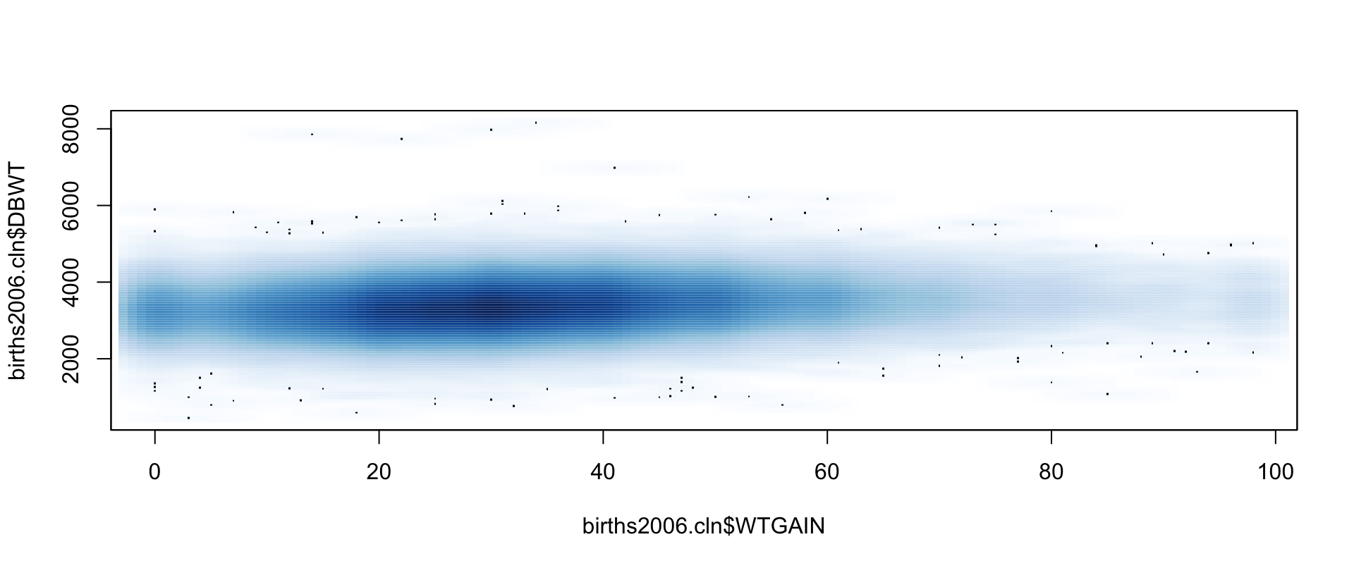
Does the mother’s weight gain correlate with the baby’s weight? Clean first (valid values, single births, gestation > 35 weeks), then look — 100k+ points need smoothScatter, not plot:
temp <- tempfile(fileext = ".rda")
download.file("https://raw.githubusercontent.com/cran/nutshell/master/data/births2006.smpl.rda",
              temp, mode = "wb")
load(temp)
births2006.cln <- births2006.smpl[
  !is.na(births2006.smpl$WTGAIN) & !is.na(births2006.smpl$DBWT) &
  births2006.smpl$DPLURAL == "1 Single" & births2006.smpl$ESTGEST>35,]
smoothScatter(births2006.cln$WTGAIN, births2006.cln$DBWT)[1] 0.1751866[1] 0.1776192A modest correlation by either measure — the blob is angled, just barely. (The book used the full 3.2M-record file; our 10% sample gives near-identical values.)
Covariance is the Pearson numerator — same arguments as cor:
Relatives: cov2cor converts a covariance matrix to a correlation matrix; cov.wt(x, wt=, cor=, center=, method=c("unbiased","ML")) computes weighted covariance.
PCA rewrites possibly-correlated variables as uncorrelated components. Two implementations: prcomp (preferred; formula method prcomp(~..., data=, subset=, na.action=), default method with retx, center=TRUE, scale., tol) and the S-PLUS-compatible princomp (eigendecomposition of the correlation/covariance matrix) — the book demonstrates the latter.
Data: team batting statistics 2000–2008, extracted from the Baseball Databank by SQL (renamed to readable play names) and packaged as team.batting.00to08:
temp <- tempfile(fileext = ".rda")
download.file("https://raw.githubusercontent.com/cran/nutshell/master/data/team.batting.00to08.rda",
              temp, mode = "wb")
load(temp)
batting.pca <- princomp(~singles+doubles+triples+homeruns+
                          walks+hitbypitch+sacrificeflies+
                          stolenbases+caughtstealing,
                        data=team.batting.00to08)
summary(batting.pca)
Importance of components:
Comp.1 Comp.2 Comp.3 Comp.4 Comp.5
Standard deviation 74.9009809 61.8710858 31.8113983 27.98819003 23.78885885
Proportion of Variance 0.4610727 0.3146081 0.0831687 0.06437897 0.04650949
Cumulative Proportion 0.4610727 0.7756807 0.8588494 0.92322841 0.96973790
Comp.6 Comp.7 Comp.8 Comp.9
Standard deviation 12.88429066 9.150840397 8.283972499 7.060503344
Proportion of Variance 0.01364317 0.006882026 0.005639904 0.004096998
Cumulative Proportion 0.98338107 0.990263099 0.995903002 1.000000000Two components already carry ~78% of the variance; four carry ~92%.
loadings shows each variable’s contribution to each component:
Loadings:
               Comp.1 Comp.2 Comp.3 Comp.4 Comp.5 Comp.6 Comp.7 Comp.8 Comp.9
singles         0.313  0.929  0.136         0.136
doubles                       0.437  0.121 -0.877                0.100
triples                                                  -0.424 -0.775  0.449
homeruns       -0.235         0.383  0.825  0.324
walks          -0.914  0.328 -0.150 -0.182
hitbypitch                                         0.989
sacrificeflies                                           -0.321 -0.330 -0.882
stolenbases            0.131 -0.758  0.502 -0.307         0.232
caughtstealing               -0.208  0.104               -0.813  0.521  0.105

               Comp.1 Comp.2 Comp.3 Comp.4 Comp.5 Comp.6 Comp.7 Comp.8 Comp.9
SS loadings     1.000  1.000  1.000  1.000  1.000  1.000  1.000  1.000  1.000
Proportion Var  0.111  0.111  0.111  0.111  0.111  0.111  0.111  0.111  0.111
Cumulative Var  0.111  0.222  0.333  0.444  0.556  0.667  0.778  0.889  1.000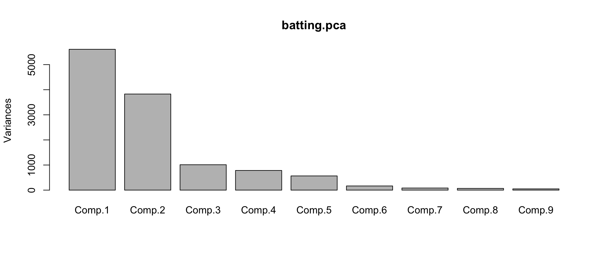
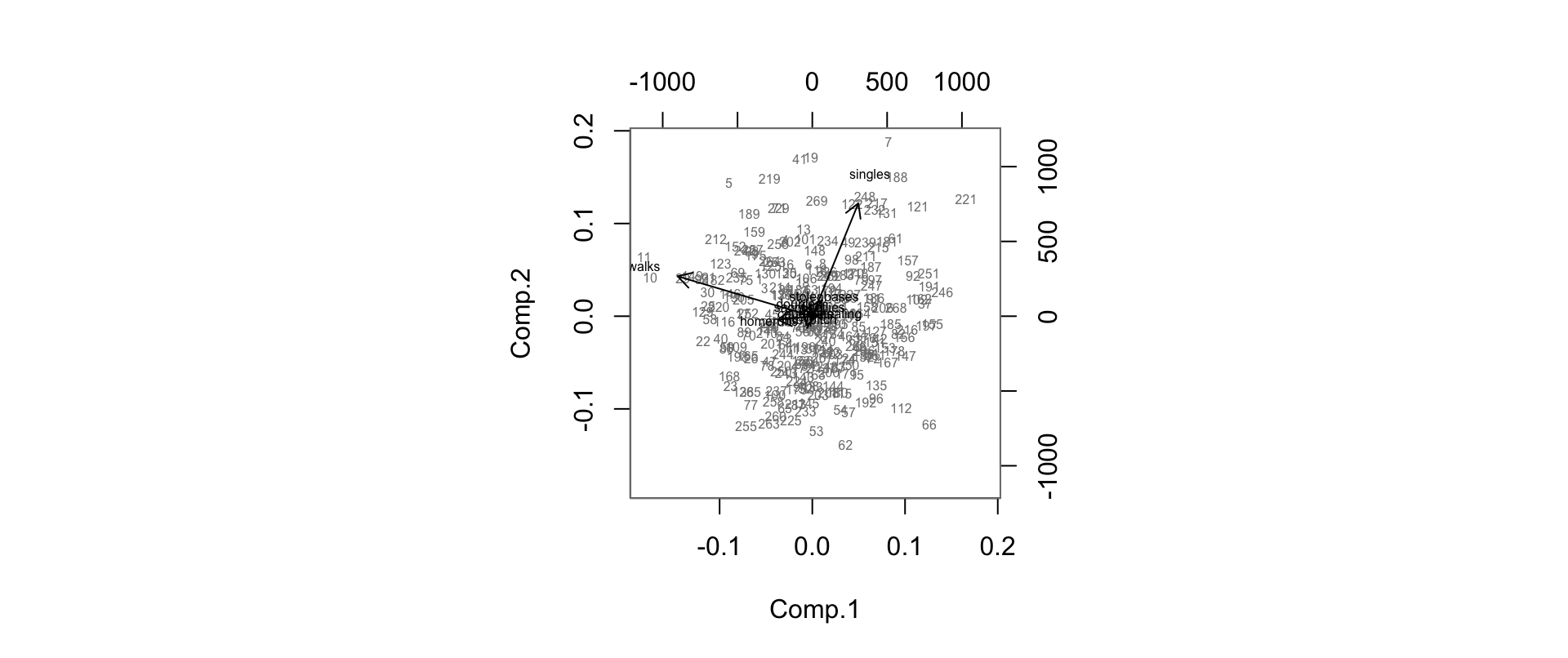
The biplot draws variable contributions to components 1–2 and the observations on one scale: singles and walks dominate the first two components. (This data returns for linear modeling in Chapter 20.)
Some quantities are observable (test scores); some are not (intelligence). Factor analysis infers hidden factors from observed variables — factanal in stats:
| Argument | Description |
|---|---|
x / data |
formula or numeric matrix (+ data frame for the formula) |
factors |
how many factors to fit |
covmat / n.obs |
alternatively: a covariance matrix (or cov.wt output) + observation count |
subset / na.action / start |
the usual suspects |
scores |
"none", "regression" (Thompson), "Bartlett" (weighted least squares) |
rotation |
factor rotation function, default "varimax" |
Is your statistic sensitive to a few outliers? What’s its sampling range? Bootstrapping answers for any statistic: repeatedly resample observations with replacement, recompute the statistic, study the spread — formally, an estimate of an estimator’s bias.
Key arguments: data; statistic — a function of (data, selection) where stype defines the second argument ("i" indices, "f" frequencies, "w" weights); R — number of replicates; sim — "ordinary", "parametric", "balanced", "permutation", "antithetic"; strata for multisample problems; ran.gen/mle for parametric simulation; simple=TRUE trades time for memory.
Media report median home prices. Bootstrapping June 2008 San Francisco sale prices:
temp <- tempfile(fileext = ".rda")
download.file("https://raw.githubusercontent.com/cran/nutshell/master/data/sanfrancisco.home.sales.rda",
              temp, mode = "wb")
load(temp)
home.sale.prices.june2008 <- subset(sanfrancisco.home.sales,
  format(date, "%Y-%m")=="2008-06")$price
library(boot)
b <- boot(data=home.sale.prices.june2008,
          statistic=function(d, i) { median(d[i]) },
          R=1000)
b
ORDINARY NONPARAMETRIC BOOTSTRAP


Call:
boot(data = home.sale.prices.june2008, statistic = function(d,
    i) {
    median(d[i])
}, R = 1000)


Bootstrap Statistics :
    original  bias    std. error
t1*   845000 -3990.5     22636.2
Verdict: the median is a very slightly biased estimator here — and now we also know its standard error, free of any normality assumption.
Copyright. These slides are adapted from R in a Nutshell: A Desktop Quick Reference (2nd ed.) by Joseph Adler, O’Reilly Media. All rights reserved by the original author and publisher.
Non-commercial use only. These materials are strictly for educational purposes and may not be used for commercial gain.
Attribution. Any reproduction, distribution, or use of these materials must properly credit the original source.

R in a Nutshell: A Desktop Quick Reference