Programming for Applications

Chapter 17: Probability Distributions

Yu-You Liou (NTU)

Shih Chien University

2026-07-20

d, p, q, r

Why Distributions Matter Here

Many statistical tests compute a test statistic, then compare it to a value from a theoretical distribution — exactly what Chapter 18 will do. R supplies, for every common distribution, functions to calculate densities, distribution functions (cumulative probabilities), quantiles, and random draws. This chapter walks through the normal distribution in detail, then catalogs the whole family.

The Normal Distribution

dnorm: the Density

\[f(x) = \frac{1}{\sigma\sqrt{2\pi}}\, e^{-\frac{(x-\mu)^2}{2\sigma^2}}\]

dnorm(x, mean=0, sd=1, log=FALSE) evaluates the density at x (log=TRUE returns its logarithm). Plotting it is one line:
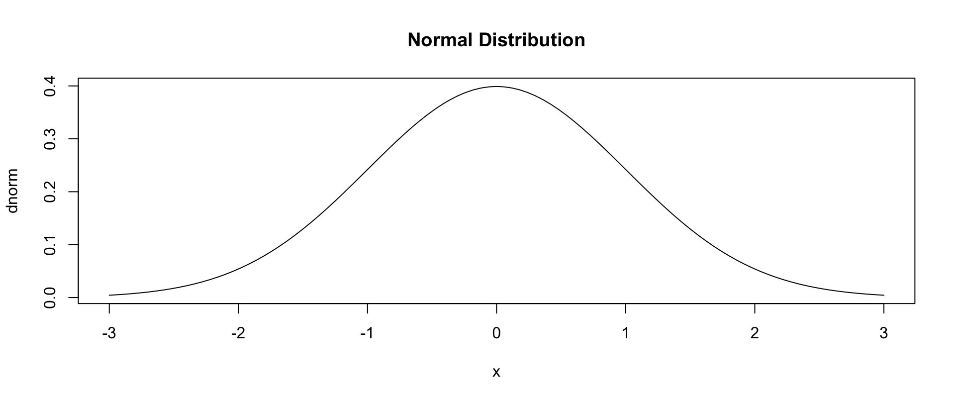
plot(dnorm, -3, 3, main = "Normal Distribution")

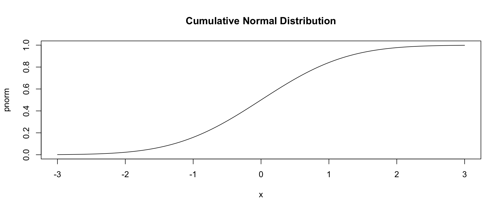
pnorm: the Distribution Function

pnorm(q, mean=0, sd=1, lower.tail=TRUE, log.p=FALSE) returns \(p = \Pr(x \le q)\) — the probability that a random value falls at or below q. lower.tail=FALSE flips to \(\Pr(x > q)\); log.p=TRUE returns \(\log(p)\):

pnorm(0)          # symmetric around 0, so exactly .5
[1] 0.5
pnorm(-1)         # below one sd under the mean
[1] 0.1586553
pnorm(1.96) - pnorm(-1.96)   # within 1.96 sd: the famous 95%
[1] 0.9500042
plot(pnorm, -3, 3, main = "Cumulative Normal Distribution")

qnorm: the Quantile Function

qnorm(p, mean=0, sd=1, lower.tail=TRUE, log.p=FALSE) is pnorm’s inverse: it returns the q for which \(p = \Pr(x \le q)\):

qnorm(0.5)                     # the median
[1] 0
qnorm(log(0.5), log.p=TRUE)
[1] 0
qnorm(pnorm(-1))               # inverse, demonstrated
[1] -1
c(qnorm(.025), qnorm(.975))    # both ends of a 95% confidence interval
[1] -1.959964  1.959964

rnorm: Random Draws

rnorm(n, mean=0, sd=1) generates n random values — for testing functions, simulations, sampling methods:
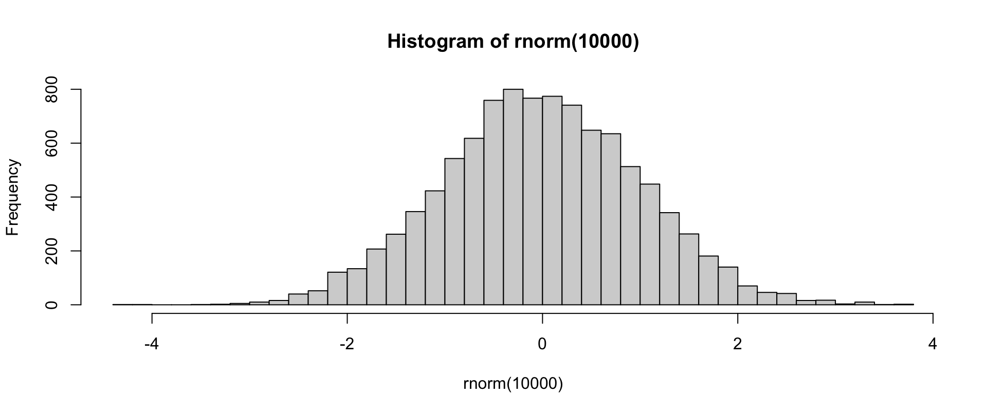

hist(rnorm(10000), breaks=50)

The Naming System

Four Prefixes, Shared Arguments

Nearly every distribution follows one convention:

  • d — probability density function (for discrete distributions, technically the probability mass function);
  • p — distribution function;
  • q — quantile function;
  • r — random number generator.

And shared arguments by type: density functions take x, log; distribution functions take q, lower.tail, log.p; quantile functions take p, lower.tail, log.p; random generators take n (renamed nn for the hypergeometric, whose parameters claimed the letter). Knowing the system, you can usually guess the function you need.

Distribution Function Families

Continuous Distributions

Family R functions Family arguments
Beta dbeta pbeta qbeta rbeta shape1, shape2, ncp=0
Cauchy dcauchy pcauchy qcauchy rcauchy location, scale
Chi-squared dchisq pchisq qchisq rchisq df, ncp=0
Exponential dexp pexp qexp rexp rate
F df pf qf rf df1, df2, ncp
Gamma dgamma pgamma qgamma rgamma shape, rate=1, scale=1/rate
Log-normal dlnorm plnorm qlnorm rlnorm meanlog, sdlog
Logistic dlogis plogis qlogis rlogis location, scale
Normal dnorm pnorm qnorm rnorm mean, sd
Student’s t dt pt qt rt df, ncp
Uniform dunif punif qunif runif min, max
Weibull dweibull pweibull qweibull rweibull shape, scale

Discrete and Special Distributions

Family R functions Family arguments
Binomial dbinom pbinom qbinom rbinom size, prob
Birthday (coincidences) pbirthday qbirthday classes, coincident
Geometric dgeom pgeom qgeom rgeom prob
Hypergeometric dhyper phyper qhyper rhyper m, n, k (random’s count is nn!)
Multinomial dmultinom rmultinom size, prob
Negative binomial dnbinom pnbinom qnbinom rnbinom size, prob, mu
Poisson dpois ppois qpois rpois lambda
Studentized range ptukey qtukey nmeans, df, nranges
Wilcoxon rank sum dwilcox pwilcox qwilcox rwilcox m, n
Wilcoxon signed rank dsignrank psignrank qsignrank rsignrank n
dbinom(3, size=10, prob=0.5)    # exactly 3 heads in 10 fair flips
[1] 0.1171875
ppois(2, lambda=4)              # at most 2 events when 4 are expected
[1] 0.2381033
qbirthday(0.5)                  # people needed for a 50% shared birthday
[1] 23

Tip

The d-p-q-r grid is your map. Test statistics (Chapter 18) live in pt/pf/pchisq; confidence intervals in qt/qnorm; simulations in r*. Whenever a formula says “compare to the χ² distribution with k degrees of freedom,” the R translation is one pchisq call.