# data sets used throughout this chapter
for (d in c("tires.sus", "field.goals", "SPECint2006",
            "mort06.smpl", "births2006.smpl")) {
  temp <- tempfile(fileext = ".rda")
  download.file(paste0("https://raw.githubusercontent.com/cran/nutshell/",
                       "master/data/", d, ".rda"), temp, mode = "wb")
  load(temp, envir = globalenv())
}Programming for Applications
Chapter 18: Statistical Tests
Yu-You Liou (NTU)
Shih Chien University
2026-08-03
Hypotheses on Trial
The Shape of the Chapter
“Does the new drug beat the placebo?” “Does the redesign sell more?” “Does this strategy beat the index?” — formulate a hypothesis, design an experiment, collect data, test. Two halves:
- continuous data — normal-theory tests, then nonparametric counterparts;
- discrete data — proportions, binomial trials, contingency tables.
Warning
The book’s own disclaimer applies here too: these slides remind you when and how to run each test in R — they are no substitute for a proper statistics course on where the formulas come from and when they’re safe.
Continuous Data: Normal-Theory Tests
t.test: One Sample Against a Hypothesized Mean
t.test(x, y=NULL, alternative=c("two.sided","less","greater"), mu=0, paired=FALSE, var.equal=FALSE, conf.level=0.95) — y=NULL compares one vector against mu; var.equal chooses pooled variance vs. the Welch method. Suppose type-H tires “should” last 9 hours:
[1] 10.182
    One Sample t-test

data:  times.to.failure.h
t = 0.75694, df = 9, p-value = 0.4684
alternative hypothesis: true mean is not equal to 9
95 percent confidence interval:
  6.649536 13.714464
sample estimates:
mean of x
   10.182
Reading it: statistic t, degrees of freedom, p-value 0.4684 — the alternative (“true mean ≠ 9”) is not supported; the evidence does not imply the mean differs from 9. The 95% CI and sample mean close the report.
t.test: Two Samples
Three tire types shared speed rating S — equal lifetimes expected. E vs. D, then E vs. B:
times.to.failure.e <- subset(tires.sus,
  Tire_Type=="E" & Speed_At_Failure_km_h==180)$Time_To_Failure
times.to.failure.d <- subset(tires.sus,
  Tire_Type=="D" & Speed_At_Failure_km_h==180)$Time_To_Failure
times.to.failure.b <- subset(tires.sus,
  Tire_Type=="B" & Speed_At_Failure_km_h==180)$Time_To_Failure
t.test(times.to.failure.e, times.to.failure.d)
    Welch Two Sample t-test

data:  times.to.failure.e and times.to.failure.d
t = -2.5042, df = 8.961, p-value = 0.03373
alternative hypothesis: true difference in means is not equal to 0
95 percent confidence interval:
 -0.82222528 -0.04148901
sample estimates:
mean of x mean of y
4.321000 4.752857 [1] 0.1639728E vs. D: significant at 95% (p = 0.034). E vs. B: not (p = 0.164) — and note R never says “significant”; you read the p-value yourself.
t.test: the Formula Interface
With data in a frame and groups in a factor: t.test(formula, data, subset, na.action). TV pundits insist outdoor kicking is harder — do successful field goals differ in distance?
    Welch Two Sample t-test

data:  yards by outside
t = 1.1259, df = 319.43, p-value = 0.261
alternative hypothesis: true difference in means between group FALSE and group TRUE is not equal to 0
95 percent confidence interval:
 -0.6851121  2.5185711
sample estimates:
mean in group FALSE  mean in group TRUE
           35.31707            34.40034
A yard longer indoors on average — not significant (p = 0.26). Misses (data=bad): p = 0.23. Attempts overall: p = 0.12. The pundits remain unvindicated.
Paired Data
Two observations per subject (before/after) call for a paired t-test: paired=TRUE. SPEC’s CPU benchmarks report a baseline and an optimized result per system — paired by machine. Single-chip dual-core systems:
    Paired t-test

data:  subset(SPECint2006, Num.Chips == 1 & Num.Cores == 2)$Baseline and subset(SPECint2006, Num.Chips == 1 & Num.Cores == 2)$Result
t = -21.804, df = 111, p-value < 2.2e-16
alternative hypothesis: true mean difference is not equal to 0
95 percent confidence interval:
 -1.957837 -1.631627
sample estimates:
mean difference
      -1.794732
Resoundingly significant — no shock: tuning helps, and submitting optimized results is voluntary.
Comparing Variances: var.test and bartlett.test
var.test(x, y, ratio=1, alternative=, conf.level=)(or formula form) runs an F-test on two normal-population variances.bartlett.test(x, g)(or formula) tests homogeneity of variance across groups.
    F test to compare two variances

data:  yards by outside
F = 1.2432, num df = 252, denom df = 728, p-value = 0.03098
alternative hypothesis: true ratio of variances is not equal to 1
95 percent confidence interval:
 1.019968 1.530612
sample estimates:
ratio of variances
          1.243157
    Bartlett test of homogeneity of variances

data:  yards by outside
Bartlett's K-squared = 4.5808, df = 1, p-value = 0.03233
Both p-values ≈ 0.03: the indoor/outdoor variance difference is significant — the means weren’t, the spreads are.
ANOVA: Comparing Many Means
Analysis of variance compares means across multiple groups (named for the method, not the result!). The quick tool is aov(formula, data, projections=, qr=, contrasts=). Age at death by cause, US 2006 (mort06.smpl, recoded by the author from CDC files):
Call:
   aov(formula = age ~ Cause, data = mort06.smpl)

Terms:
                   Cause Residuals
Sum of Squares  15727886  72067515
Deg. of Freedom        9    243034

Residual standard error: 17.22012
Estimated effects may be unbalanced
因為不存在,29 個觀察量被刪除了
model.tables(aov(...)) prints per-level effects (Accidents −21.4 years vs. overall, Homicide −40.1, Alzheimer’s +13.8…). A subtler example — weight gain by birth month:
Call:
   aov(formula = WTGAIN ~ DOB_MM, data = births2006.cln)

Terms:
                  DOB_MM Residuals
Sum of Squares     14777  73385301
Deg. of Freedom        1    351465

Residual standard error: 14.44986
Estimated effects may be unbalanced
anova(lm(…)), oneway.test, and Friends
The often-better route: fit with lm, extract the table with anova — F-statistic and p-value included (and update modifies big models cheaply; Chapter 20):
Analysis of Variance Table

Response: age
              Df   Sum Sq Mean Sq F value    Pr(>F)
Cause          9 15727886 1747543  5893.3 < 2.2e-16 ***
Residuals 243034 72067515     297
---
Signif. codes: 0 '***' 0.001 '**' 0.01 '*' 0.05 '.' 0.1 ' ' 1- Variances unequal?
oneway.test(formula, data, var.equal=FALSE)— the Welch idea, generalized. - More
aovaccessories:proj(projections),TukeyHSD(CIs on pairwise level differences),se.contrast(standard errors of contrasts).
Pairwise t-Tests
Want which groups differ, not just whether: pairwise.t.test(x, g, p.adjust.method=, pool.sd=, paired=, alternative=) runs all pairs with multiple-testing correction (default: Holm):
    Pairwise comparisons using t tests with pooled SD

data:  tires.sus$Time_To_Failure and tires.sus$Tire_Type

  B       C      D       E       H
C 0.2219  -      -       -       -
D 1.0000  0.5650 -       -       -
E 1.0000  0.0769 1.0000  -       -
H 2.4e-07 0.0029 2.6e-05 1.9e-08 -
L 0.1147  1.0000 0.4408  0.0291  0.0019

P value adjustment method: holm
No significant difference for C–L, D–L, D–E; very significant for B–H, C–H, E–L…
Testing Normality: shapiro.test
Are field-goal distances normal? Eyeball first, then the Shapiro-Wilk test:
    Shapiro-Wilk normality test

data:  field.goals$yards
W = 0.97275, p-value = 1.309e-12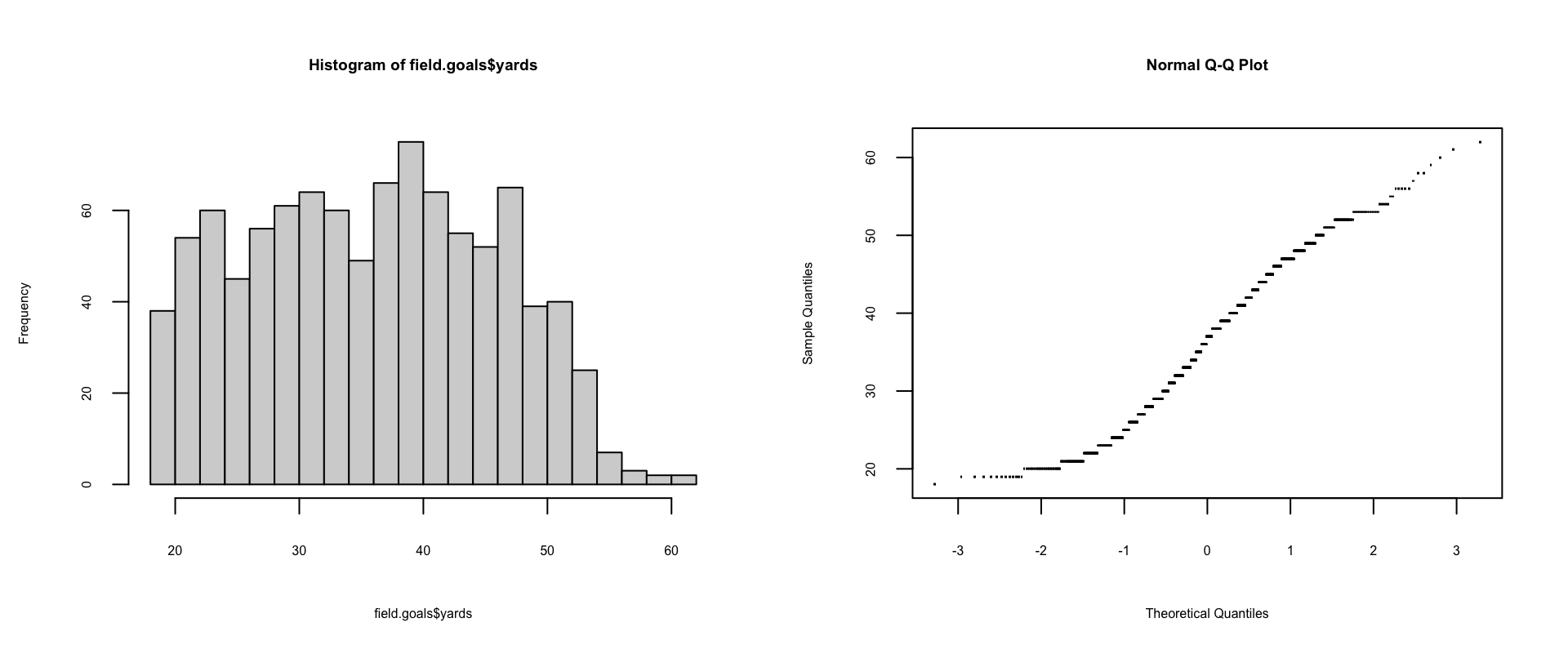
Bell-ish shape, roughly linear Q-Q — yet p ≈ 10⁻¹²: quite likely not normal. Eyes deceive; tests quantify.
Arbitrary Distributions: ks.test
The Kolmogorov-Smirnov test compares a vector to any distribution (y = data vector, distribution name, or function), or two vectors to each other:
Warning in ks.test.default(field.goals$yards, pnorm): ties should not be
present for the one-sample Kolmogorov-Smirnov test
    Asymptotic one-sample Kolmogorov-Smirnov test

data:  field.goals$yards
D = 1, p-value < 2.2e-16
alternative hypothesis: two-sided
    Asymptotic two-sample Kolmogorov-Smirnov test

data:  jitter(subset(SPECint2006, Num.Chips == 1 & Num.Cores == 2)$Baseline) and jitter(subset(SPECint2006, Num.Chips == 1 & Num.Cores == 2)$Result)
D = 0.20536, p-value = 0.01777
alternative hypothesis: two-sided
The ties warning is itself informative — true normal values almost never tie. (We jitter the second test to silence it.) Baseline and optimized results: unlikely to share a distribution (p = 0.012).
Correlation Tests: cor.test
Chapter 16’s cor gives a number; cor.test(x, y, alternative=, method=, exact=, conf.level=) (or formula form) gives significance:
[1] 2.989378e-08[1] 0.2671036The Chapter 13 toxins-and-lung-cancer relationship, tested:
    Pearson's product-moment correlation

data:  air_on_site/Surface_Area and deaths_lung/Population
t = 3.4108, df = 39, p-value = 0.00152
alternative hypothesis: true correlation is not equal to 0
95 percent confidence interval:
 0.2013723 0.6858402
sample estimates:
      cor
0.4793273
Significant positive correlation (p = 0.0015) — but resist the causal leap: industrial states may differ in income, healthcare, smoking, or even death-certificate habits.
Continuous Data: Nonparametric Tests
wilcox.test
When normality is doubtful, rank-based tests trade some power for robustness. The Wilcoxon test is the t-test’s counterpart: its statistic counts, over all pairs, how often y[j] < x[i] (about half if the distributions match); for the one-sample-vs-location analogue, pass a single sample with mu= (the Wilcoxon signed-rank test):
    Wilcoxon rank sum exact test

data:  times.to.failure.e and times.to.failure.d
W = 14.5, p-value = 0.04576
alternative hypothesis: true location shift is not equal to 0
    Wilcoxon rank sum test with continuity correction

data:  yards by outside
W = 62045, p-value = 0.393
alternative hypothesis: true location shift is not equal to 0
Note the contrast with the t-test: E vs. D barely misses significance here (p = 0.0505). Ties trigger a normal approximation (hence the warning).
kruskal.test and fligner.test
- Kruskal-Wallis rank-sum test — nonparametric ANOVA:
kruskal.test(formula, data); - Fligner-Killeen (median) test — nonparametric variance comparison:
fligner.test(formula, data).
    Kruskal-Wallis rank sum test

data:  age by Cause
Kruskal-Wallis chi-squared = 34868, df = 9, p-value < 2.2e-16
    Fligner-Killeen test of homogeneity of variances

data:  age by Cause
Fligner-Killeen:med chi-squared = 15788, df = 9, p-value < 2.2e-16- Scale-parameter differences:
ansari.test(x, y, ...)(Ansari-Bradley) andmood.test(x, y, ...)(Mood) — both with formula variants.
Discrete Data
prop.test: Comparing Proportions
prop.test(x, n, p=NULL, alternative=, conf.level=, correct=) tests whether success proportions differ across groups (or equal given values). Is field-goal success equal indoors and out? Build a successes/failures table (dropping the 8 aborted and 24 blocked kicks), transpose, test:
       FG good FG no
  Both      53    14
  In       152    24
  Out      582   125
    3-sample test for equality of proportions without continuity correction

data:  field.goals.table.t
X-squared = 2.3298, df = 2, p-value = 0.312
alternative hypothesis: two.sided
sample estimates:
   prop 1    prop 2    prop 3
0.7910448 0.8636364 0.8231966
p = 0.31: no significant difference in success rates among Both/In/Out.
binom.test: Bernoulli Trials
A series of identical two-outcome trials (coin flips) follows the binomial distribution. binom.test(x, n, p=0.5, alternative=, conf.level=) tests an observed success count. David Ortiz hit .264 (110/416) in 2008 — if he were “truly” a .300 hitter, how likely is hitting .264 or worse?
    Exact binomial test

data:  110 and 416
number of successes = 110, number of trials = 416, p-value = 0.06174
alternative hypothesis: true probability of success is less than 0.3
95 percent confidence interval:
 0.0000000 0.3023771
sample estimates:
probability of success
             0.2644231
p = 0.062: about a 6% chance. Notable: this p-value is the probability of being at least as far in the stated direction — read alternative carefully.
fisher.test: Exact Independence Testing
For contingency tables, the hypothesis is independence of the two variables. For small tables, Fisher’s exact test is best. Arguments: x (matrix or factor), y (factor when x is), workspace, hybrid (approximate for >2×2), or (hypothesized odds ratio), alternative, conf.int/conf.level, simulate.p.value/B (Monte Carlo). Delivery method × sex, July 2006:
    C-section Vaginal
  F      5326   12622
  M      6067   13045
    Fisher's Exact Test for Count Data

data:  method.and.sex
p-value = 1.604e-05
alternative hypothesis: true odds ratio is not equal to 1
95 percent confidence interval:
 0.8678345 0.9485129
sample estimates:
odds ratio
 0.9072866
Tiny p-value: reject independence — the sex mix differs by delivery method (girls are 46.7% of C-section deliveries vs. 49.2% of vaginal ones; odds ratio ≈ 0.91).
fisher.test on Twins; chisq.test
For twins only, the story reverses:
[1] 0.6699808p = 0.67: independence is plausible. Fisher’s test gets expensive for large tables — the workhorse alternative is the chi-squared test, which compares the sample to hypothesized probabilities (chisq.test(x, y=, correct=, p=, rescale.p=, simulate.p.value=, B=)):
chisq.test: Goodness of Fit, Higher Dimensions
Births by weekday — could the weekend deficit be chance, if every day were equally likely (the default p)?
    1     2     3     4     5     6     7
40274 62757 69775 70290 70164 68380 45683
    Chi-squared test for given probabilities

data:  births2006.byday
X-squared = 15873, df = 6, p-value < 2.2e-16
Emphatically not chance (though with n this big, everything is significant). Multidimensional tables work too — day × month:
    Pearson's Chi-squared test

data:  table(births2006.smpl$DOB_WK, births2006.smpl$DOB_MM)
X-squared = 4729.6, df = 66, p-value < 2.2e-16- Three-way interactions:
mantelhaen.test(x, y, z, ...)(Cochran-Mantel-Haenszel). - Symmetry of a 2-D table:
mcnemar.test(x, y, correct=).
friedman.test
The Friedman rank-sum test is the nonparametric counterpart of two-way ANOVA — friedman.test(y, groups, blocks) or the formula/table forms:
    Friedman rank sum test

data:  method.and.sex.twins
Friedman chi-squared = 2, df = 1, p-value = 0.1573
Agreeing with the chi-squared verdict: no significant association is detected — though remember, a non-significant p-value fails to reject independence; it does not prove it.
Copyright Notice
Copyright. These slides are adapted from R in a Nutshell: A Desktop Quick Reference (2nd ed.) by Joseph Adler, O’Reilly Media. All rights reserved by the original author and publisher.
Non-commercial use only. These materials are strictly for educational purposes and may not be used for commercial gain.
Attribution. Any reproduction, distribution, or use of these materials must properly credit the original source.

R in a Nutshell: A Desktop Quick Reference