This chapter starts with the simplest model — linear regression by ordinary least squares (OLS) — then builds, evaluates, refines it, and surveys richer model types. Classification waits for Chapter 21.
A Simple Linear Model
The Data and the Question
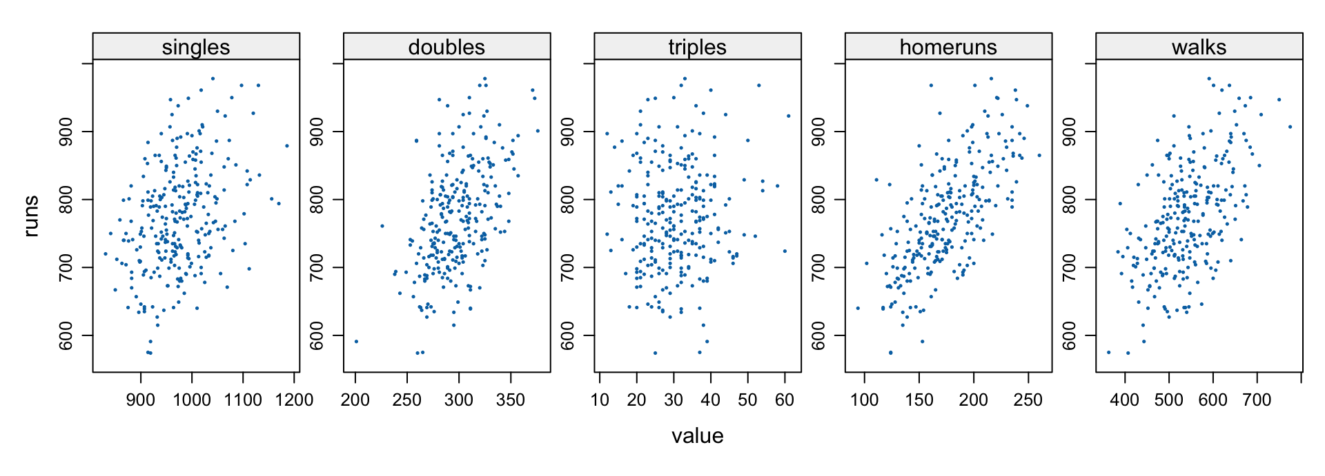
Which batting metrics predict a team’s runs? Team batting 2000–2008 (extracted by SQL in Chapter 16, packaged as team.batting.00to08):
lm fits a linear model by OLS. Note: in formulas + * - ^ are special; wrap literal arithmetic in I(), and generate polynomial terms with poly(x, degree=).
anova(model1, model2, ...) compares nested models; update(model, formula) refits after a formula change — far cheaper than building from scratch on large data.
Diagnostic Plots
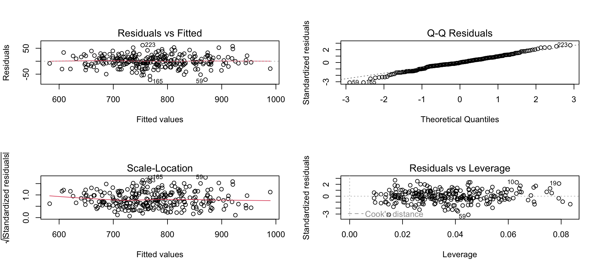
plot(lm.object) draws the standard diagnostics — residuals vs. fitted, a normal Q-Q of residuals, scale-location, and residuals vs. leverage:
par(mfrow=c(2,2))plot(runs.mdl)
par(mfrow=c(1,1))
Look for: structure in residuals (nonlinearity), departures from the Q-Q line (non-normality), a fanning scale-location (heteroscedasticity), and high-leverage outliers.
lm in Detail
lm(formula, data, subset, weights, na.action,method ="qr", model =TRUE, x =FALSE, y =FALSE,qr =TRUE, singular.ok =TRUE, contrasts =NULL, offset, ...)
The model is \(y = c_0 + c_1 x_1 + \cdots + c_n x_n + \varepsilon\); OLS chooses the \(c_i\) minimizing the sum of squared residuals. Key arguments: formula (required); data, subset, weights, na.action; contrasts controls factor coding (treatment, Helmert, …); weights gives weighted least squares. Companions glm, nls, loess, rlm share many of these argument names.
When OLS Isn’t Enough
Assumptions and Their Tests
OLS is technically valid only under assumptions — yet often predicts well even when they’re bent:
linearity of the response in the predictors;
constant error variance (homoscedasticity) — test with car::ncvTest (non-constant variance score test);
predictors not collinear (singular fits);
normally distributed, independent errors.
When they fail badly, reach for the alternatives below.
Robust and Resistant Regression
Outliers wreck OLS. Two defenses (package MASS):
Resistant regression — lqs (least trimmed squares, least median of squares): fits using a subset of points, ignoring extreme ones;
Robust regression — rlm: M-estimation, down-weighting (rather than discarding) large residuals iteratively.
Lasso / least angle regression — lars::lars(x, y, type=c("lasso","lar","forward.stagewise","stepwise")) (L1 penalty) shrinks and selects, zeroing some coefficients; it computes the entire path at once.
Ridge and lasso are both penalized regression; the modern unified tool is glmnet.
step(runs.mdl) # stepwise by AICMASS::lm.ridge(runs~., team.batting.00to08, lambda=seq(0,1,0.1))
Principal Components and PLS Regression
When predictors are many and correlated, regress on components instead — package pls, both via mvr (aliases pcr, plsr):
Principal components regression (pcr) — regress on the leading principal components of the predictors;
Partial least squares (plsr) — components chosen to also correlate with the response.
Generalized and Nonlinear Models
glm: Generalized Linear Models
glm extends linear models to non-normal responses via a family and a link function — predicting the link of the expected response:
bagging, boosting (gbm), random forests (randomForest) — ensembles of trees, each highly parallelizable (Chapter 26);
PRIM (patient rule induction method) — bump hunting.
Tip
A workflow, not a function. Fit with lm, readsummary, look at plot, then iterate with update — adding, dropping, or transforming terms. Reach for robust/penalized/nonlinear tools only when the diagnostics demand it.
Copyright Notice
Copyright. These slides are adapted from R in a Nutshell: A Desktop Quick Reference (2nd ed.) by Joseph Adler, O’Reilly Media. All rights reserved by the original author and publisher.
Non-commercial use only. These materials are strictly for educational purposes and may not be used for commercial gain.
Attribution. Any reproduction, distribution, or use of these materials must properly credit the original source.