Chapter 22: Machine Learning
Shih Chien University
2026-07-20
Chapters 20–21 were supervised — predict a known response. This chapter covers two unsupervised tasks, where there is no response to predict, only structure to discover:
Given a set of transactions (a shopping basket, a listening history), association-rule mining finds items frequently associated with each other — “customers who bought X also bought Y.” The classic algorithm is a priori, in package arules:
data — a transactions object (or a matrix/data frame coercible to one);parameter — thresholds, chiefly support (how often items appear together) and confidence (how reliable the rule is);appearance constrains which items may appear on each side; control tunes the algorithm.arules is built on S4 classes (a transactions class for the data) and the well-engineered apriori C implementation by Christian Borgelt.
The book mines Audioscrobbler listening data (now part of Last.fm). Load with read.transactions, mine, inspect:
Resulting rules read like “listeners of Green Day and Nirvana also listen to Red Hot Chili Peppers,” each with support, confidence, and lift (how much more often than chance). A related, faster algorithm for frequent itemsets is eclat.
Clustering groups observations so that members of a cluster are more similar to each other than to outsiders — and similarity starts with distance. stats::dist builds a distance matrix:
method may be "euclidean", "manhattan", "maximum", "canberra", "binary", or "minkowski" (with parameter p). The right metric matters: scale and units shape every cluster that follows, so standardize variables first when they differ in range.
Partitioning algorithms split data into a chosen number k of clusters:
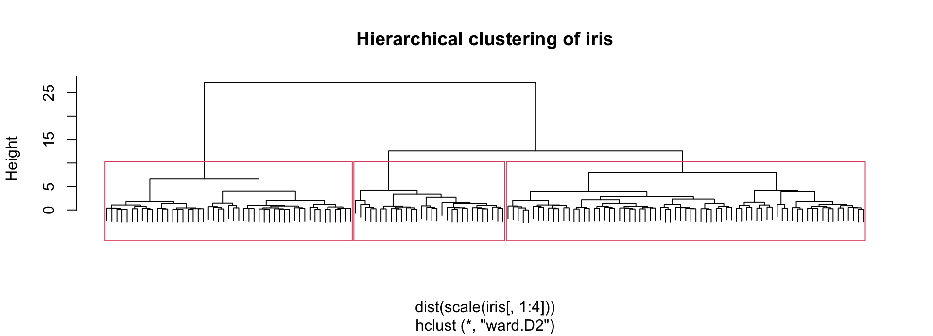
kmeans(x, centers, ...) — fast, minimizes within-cluster sum of squares; sensitive to outliers and starting centers.cluster::pam(x, k) — partitioning around medoids; uses actual data points as centers, more robust than k-means.cluster::clara(x, k) — pam scaled to large data via sampling.cluster::silhouette measures how well each point fits its cluster (−1 to 1); the average silhouette width helps choose k.k up front — hclust(dist_object, method=) builds a tree (dendrogram), merging closest clusters step by step; cluster::agnes (agglomerative) and diana (divisive) are richer alternatives.method ranges over "complete", "average", "single", "ward.D2", … — each defining “distance between clusters” differently, and each producing differently shaped clusters.
Tip
Unsupervised work has no answer key. There is no accuracy to optimize — only structure to judge. Vary the distance metric, the algorithm, and k; validate with silhouette widths, domain knowledge, and whether the clusters are useful, not merely whether they exist.

Copyright. These slides are adapted from R in a Nutshell: A Desktop Quick Reference (2nd ed.) by Joseph Adler, O’Reilly Media. All rights reserved by the original author and publisher.
Non-commercial use only. These materials are strictly for educational purposes and may not be used for commercial gain.
Attribution. Any reproduction, distribution, or use of these materials must properly credit the original source.
R in a Nutshell: A Desktop Quick Reference