Chapter 23: Time Series Analysis
Shih Chien University
2026-08-02
Time series carry long-term trends and periodic patterns that ordinary summary statistics miss. Analyzing them needs tools that respect order and lag. We revisit the turkey-price series from Chapter 7:
The autocorrelation function measures how correlated a series is with its own past, by lag — the signature of seasonality and cycles:
Autocorrelations of series 'turkey.price.ts', by lag
0.0000 0.0833 0.1667 0.2500 0.3333 0.4167 0.5000 0.5833 0.6667 0.7500 0.8333
1.000 0.465 -0.019 -0.165 -0.145 -0.219 -0.215 -0.122 -0.136 -0.200 -0.016
0.9167 1.0000 1.0833 1.1667 1.2500 1.3333 1.4167 1.5000 1.5833
0.368 0.723 0.403 -0.013 -0.187 -0.141 -0.180 -0.226 -0.130
acf plots by default; plot=FALSE returns the numbers.pacf (partial autocorrelation) — correlation at a lag after removing the influence of shorter lags; it helps identify the order of an AR model.The turkey series shows strong positive autocorrelation at 12-month lags, negative at 6 — clear annual seasonality.
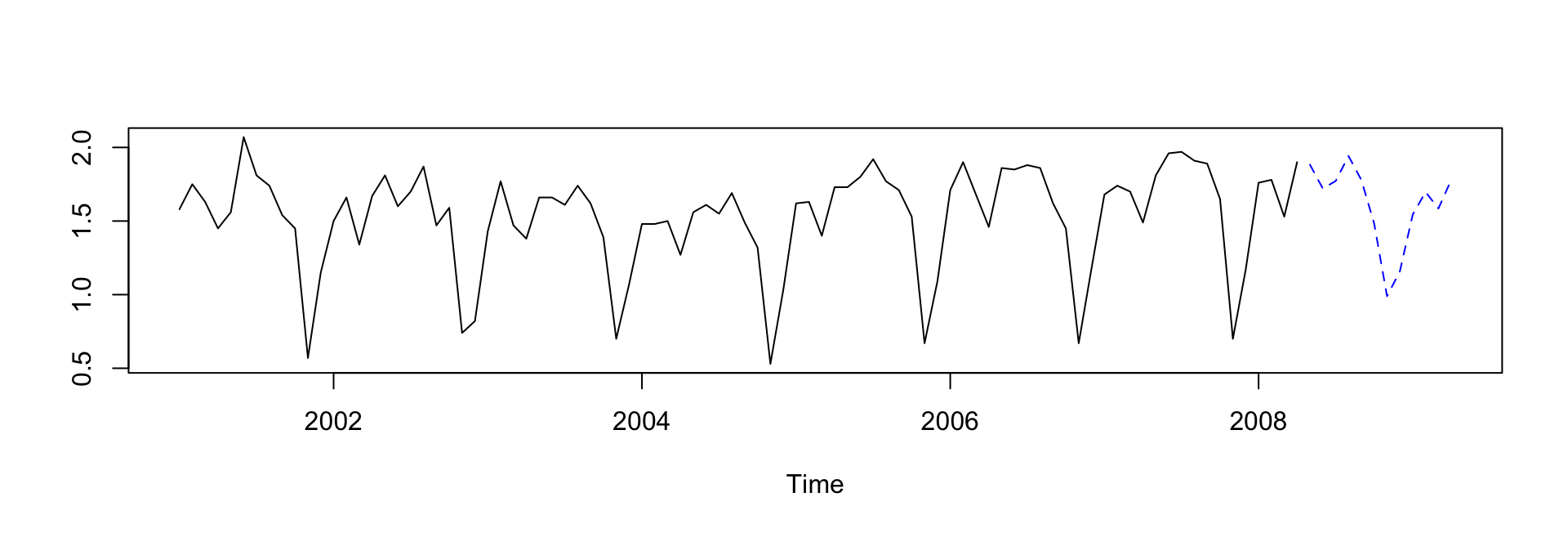
Time-series models predict future values from past ones. The autoregressive (AR) model regresses each value on its predecessors — ar even picks the order automatically by AIC:
aic=TRUE selects the order; order.max caps it; method chooses the estimation algorithm.predict on an ar object projects future values, with standard errors:
Jan Feb Mar Apr May Jun Jul
2008 1.8827277 1.7209182 1.7715016
2009 1.5439290 1.6971933 1.5849406 1.7800358
Aug Sep Oct Nov Dec
2008 1.9416776 1.7791961 1.4822070 0.9894343 1.1588863
2009
For richer dynamics, arima fits autoregressive integrated moving-average models — the order (p, d, q) capturing AR terms, differencing, and MA terms; seasonal terms extend it to SARIMA:
Call:
arima(x = turkey.price.ts, order = c(1, 0, 0), seasonal = list(order = c(1,
0, 0), period = 12))
Coefficients:
ar1 sar1 intercept
0.1744 0.8596 1.5741
s.e. 0.1127 0.0475 0.0956
sigma^2 estimated as 0.02875: log likelihood = 23.22, aic = -38.44
May Jun Jul Aug Sep Oct
2008 1.846322 1.917925 1.916521 1.863201 1.845705 1.639351
Supporting tools: diff (differencing to remove trend), Box.test (testing residual autocorrelation), HoltWinters (exponential smoothing), StructTS (structural models), and decompose/stl (splitting a series into trend, seasonal, and remainder).
Tip
The Box-Jenkins rhythm. Plot the series; check acf/pacf; difference until stationary; fit an arima; check that the residuals look like white noise (acf, Box.test); then forecast. The modern forecast and fable packages automate much of this (auto.arima).
The book closes by pointing onward: time series feed into broader analyses — regression with lagged predictors, volatility models (GARCH, package tseries), and multivariate series (VAR). The ts class (Chapter 7) is the common substrate; specialized classes like zoo and xts handle irregular spacing and richer date indexing.
Copyright. These slides are adapted from R in a Nutshell: A Desktop Quick Reference (2nd ed.) by Joseph Adler, O’Reilly Media. All rights reserved by the original author and publisher.
Non-commercial use only. These materials are strictly for educational purposes and may not be used for commercial gain.
Attribution. Any reproduction, distribution, or use of these materials must properly credit the original source.
R in a Nutshell: A Desktop Quick Reference