Statistics

Chapter 12: Analysis of Variance

Yu-You Liou

Shih Chien University

2026-10-08

Overview

Chapter 12 is about the analysis of variance (ANOVA) — an F test that compares three or more means by comparing two estimates of the same population variance.

Section	Topics
12-1	One-way ANOVA; why not multiple t tests; F = s_B^2 / s_W^2; d.f.N. = k-1, d.f.D. = N-k; summary table
12-2	Scheffé test, F' = (k-1)(C.V.); Tukey q test; Bonferroni adjustment; which test to use
12-3	Two-way ANOVA; factors, levels, treatment groups; main and interaction effects; ordinal vs. disordinal

Chapter Objectives

After completing this chapter, you should be able to

1. Use the one-way ANOVA technique to determine if there is a significant difference among three or more means.
2. Determine which means differ, using the Scheffé, Tukey, or Bonferroni tests if the null hypothesis is rejected in the ANOVA.
3. Use the two-way ANOVA technique to determine if there is a significant difference in the main effects or interaction.

Introduction

The F test of Chapter 9, which compares two variances, can also be used to compare three or more means. This technique is called the analysis of variance, or ANOVA.

The z and t tests should not be used when three or more means are compared. For three groups, the F test can show only whether a difference exists among the three means; it cannot reveal where the difference lies — between \bar{X}_1 and \bar{X}_2, \bar{X}_1 and \bar{X}_3, or \bar{X}_2 and \bar{X}_3. Other tests, such as the Scheffé, Tukey and Bonferroni tests, are used to locate the difference.

One-Way and Two-Way ANOVA

The analysis of variance used to compare three or more means is called a one-way analysis of variance, since it involves only one variable. When the study involves two variables, a two-way analysis of variance is used (Section 12-3).

Section 12-1: One-Way Analysis of Variance

Analysis of Variance

One-Way Analysis of Variance

The one-way analysis of variance test is used to test the equality of three or more means using sample variances.

The procedure is called one-way because there is only one independent variable that distinguishes between the different populations in the study. The independent variable is also called a factor.

Why Not Multiple t Tests?

At first glance it might seem that three or more sample means could be compared with multiple t tests, two means at a time. There are three reasons why this should not be done.

Three Reasons

1. The other means are ignored. When two means are compared at a time, the rest of the means under study are ignored. With the F test, all the means are compared simultaneously.
2. The type I error rate increases. The more t tests that are conducted, the greater the likelihood of getting significant differences by chance alone, so the probability of rejecting a true null hypothesis is increased. As the number of populations compared increases, the probability of making a type I error at a given \alpha also increases.
3. The number of tests explodes. Comparing 3 means two at a time requires 3 t tests; 5 means require 10 tests; 10 means require 45 tests.

Characteristics of the F Distribution

Recall from Chapter 9

1. The values of F cannot be negative, because variances are always positive or zero.
2. The distribution is positively skewed.
3. The mean value of F is approximately equal to 1.
4. The F distribution is a family of curves based on the degrees of freedom of the variance of the numerator and the degrees of freedom of the variance of the denominator.

Even though three or more means are being compared, variances are used in the test.

Two Estimates of the Population Variance

Between-Group and Within-Group Variance

The between-group variance is the first estimate of the population variance; it involves finding the variance of the means.

The within-group variance is the second estimate; it is made by computing the variance using all the data and is not affected by differences in the means.

Two Estimates of the Population Variance (cont.)

• If there is no difference in the means, the between-group estimate is approximately equal to the within-group estimate, the F test statistic is approximately 1, and H_0 is not rejected.
• When the means differ significantly, the between-group variance is much larger than the within-group variance, F is significantly greater than 1, and H_0 is rejected.

F = \frac{\text{variance between groups}}{\text{variance within groups}}

Formulas for the F Test

Grand Mean, s_B^2 and s_W^2

The grand mean \bar{X}_{GM} is the mean of all the values in all of the samples:

\bar{X}_{GM} = \frac{\sum X}{N}

The between-group variance is the variance among the means, using the sample sizes as weights:

s_B^2 = \frac{\sum n_i (\bar{X}_i - \bar{X}_{GM})^2}{k - 1}

The within-group variance is a weighted average of the individual sample variances; it does not involve differences of means:

s_W^2 = \frac{\sum (n_i - 1) s_i^2}{\sum (n_i - 1)}

where k is the number of groups, n_i is a sample size, \bar{X}_i a sample mean and s_i^2 a sample variance.

The F Test Statistic

Formula for the F Test for One-Way Analysis of Variance

F = \frac{s_B^2}{s_W^2}

where s_B^2 is the between-group variance and s_W^2 is the within-group variance.

Hypotheses for the ANOVA

H_0: \mu_1 = \mu_2 = \cdots = \mu_k H_1: \text{At least one mean is different from the others}

A significant test statistic means there is a high probability that the difference in means is not due to chance, but it does not indicate where the difference lies.

Degrees of Freedom

d.f.N. and d.f.D.

d.f.N. = k - 1 \qquad d.f.D. = N - k

where k is the number of groups and N = n_1 + n_2 + \cdots + n_k is the sum of the sample sizes.

The sample sizes need not be equal. The F test to compare means is always right-tailed.

Table 12-1: Analysis of Variance Summary Table

Table 12-1 — Analysis of Variance Summary Table

Source	Sum of squares	d.f.	Mean square	F
Between groups	SSB	k-1	MSB
Within groups (error)	SSW	N-k	MSW
Total

SSB = \sum n_i (\bar{X}_i - \bar{X}_{GM})^2 \qquad SSW = \sum (n_i - 1) s_i^2

MSB = s_B^2 = \frac{SSB}{k-1} \qquad MSW = s_W^2 = \frac{SSW}{N-k} \qquad F = \frac{s_B^2}{s_W^2} = \frac{MSB}{MSW}

SSB is the sum of squares between groups, SSW the sum of squares within groups (the error sum of squares), and MSB, MSW the mean squares.

Assumptions for the F Test

Assumptions for the F Test for Comparing Three or More Means

1. The populations from which the samples were obtained must be normally or approximately normally distributed.
2. The samples must be independent of one another.
3. The variances of the populations must be equal.
4. The samples must be simple random samples, one from each of the populations.

In this book the assumptions are stated in the exercises; in other situations you must check that they have been met before proceeding.

Procedure Table

Finding the F Test Statistic for the Analysis of Variance

Step 1. Find the mean and variance of each sample: (\bar{X}_1, s_1^2), (\bar{X}_2, s_2^2), \ldots, (\bar{X}_k, s_k^2).

Step 2. Find the grand mean: \bar{X}_{GM} = \dfrac{\sum X}{N}.

Step 3. Find the between-group variance: s_B^2 = \dfrac{\sum n_i (\bar{X}_i - \bar{X}_{GM})^2}{k-1}.

Step 4. Find the within-group variance: s_W^2 = \dfrac{\sum (n_i - 1)s_i^2}{\sum (n_i - 1)}.

Step 5. Find the F test statistic: F = \dfrac{s_B^2}{s_W^2}, with d.f.N. = k-1 and d.f.D. = N-k.

The Five-Step Procedure

The One-Way ANOVA Follows the Regular Hypothesis-Testing Procedure

Step 1. State the hypotheses.

Step 2. Find the critical values.

Step 3. Compute the test statistic.

Step 4. Make the decision.

Step 5. Summarize the results.

Example 12-1

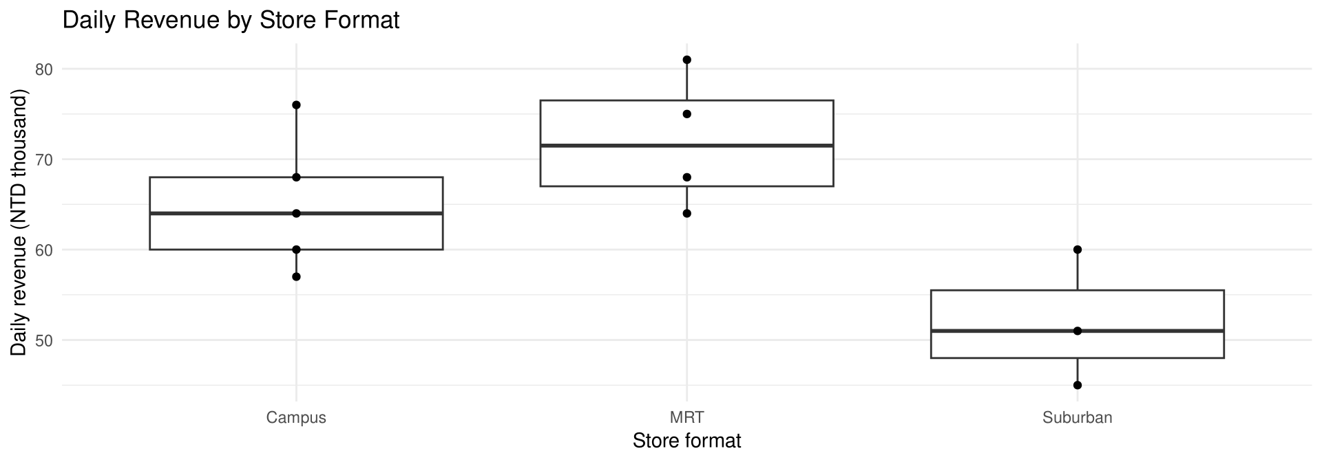
Daily Revenue by Store Format

A retail analyst at a Taipei beverage chain wishes to see if there is a difference in mean daily revenue among three store formats: MRT-station kiosks, campus outlets and suburban drive-through stores. She randomly samples four MRT kiosks, five campus outlets and three suburban stores and records one day’s revenue (NTD thousand) at each. At \alpha = 0.05, test the claim that there is no difference among the means.

MRT       Campus    Suburban
 81         76          60
 75         68          51
 68         64          45
 64         60
            57

(hypothetical data)

Back to Example 12-3 · Back to Example 12-5

Example 12-1

Solution

Step 1. State the hypotheses and identify the claim.

H_0: \mu_1 = \mu_2 = \mu_3 \ \textit{(claim)} H_1: \text{At least one mean is different from the others}

Step 2. Find the critical value. With N = 12 and k = 3,

d.f.N. = k - 1 = 3 - 1 = 2 \qquad d.f.D. = N - k = 12 - 3 = 9

The critical value from Table A-7 with \alpha = 0.05 is 4.26.

qf(0.95, df1 = 2, df2 = 9)   # Table A-7 rounds this value to 4.26

[1] 4.256495

Example 12-1

Solution

Step 3a-b — the group statistics and the grand mean

mrt_kiosks <- c(81, 75, 68, 64)
campus     <- c(76, 68, 64, 60, 57)
suburban   <- c(60, 51, 45)

mean(mrt_kiosks)

[1] 72

mean(campus)

[1] 65

mean(suburban)

[1] 52

var(mrt_kiosks)

[1] 56.66667

var(campus)

[1] 55

var(suburban)

[1] 57

mean(c(mrt_kiosks, campus, suburban))

[1] 64.08333

Example 12-1

Solution

Step 3c-e — the two variance estimates and F

s_B^2 = \frac{4(72 - 64.083)^2 + 5(65 - 64.083)^2 + 3(52 - 64.083)^2}{3-1} = \frac{692.917}{2} = 346.458

s_W^2 = \frac{(4-1)(56.667) + (5-1)(55) + (3-1)(57)}{(4-1)+(5-1)+(3-1)} = \frac{504}{9} = 56

F = \frac{s_B^2}{s_W^2} = \frac{346.458}{56} = 6.187

between_var <- (4 * (72 - 64.08333)^2 + 5 * (65 - 64.08333)^2 +
                3 * (52 - 64.08333)^2) / (3 - 1)
within_var  <- ((4 - 1) * 56.66667 + (5 - 1) * 55 + (3 - 1) * 57) /
               ((4 - 1) + (5 - 1) + (3 - 1))

between_var

[1] 346.4583

within_var

[1] 56

between_var / within_var

[1] 6.186756

Example 12-1

Solution

Steps 4-5 — the decision and the summary

Step 4. The test statistic 6.187 > 4.26, so the decision is to reject the null hypothesis.

Step 5. There is enough evidence to conclude that at least one mean is different from the others.

revenue <- data.frame(
  daily_revenue = c(mrt_kiosks, campus, suburban),
  store_format  = rep(c("MRT", "Campus", "Suburban"), times = c(4, 5, 3))
)

summary(aov(daily_revenue ~ store_format, data = revenue))

             Df Sum Sq Mean Sq F value Pr(>F)  
store_format  2  692.9   346.5   6.187 0.0204 *
Residuals     9  504.0    56.0                 
---
Signif. codes:  0 '***' 0.001 '**' 0.01 '*' 0.05 '.' 0.1 ' ' 1

Example 12-1

Solution

Table 12-2 — Analysis of Variance Summary Table for Example 12-1

Source	Sum of squares	d.f.	Mean square	F
Between groups	692.917	2	346.458	6.187
Within groups (error)	504.000	9	56.000
Total	1196.917	11

In Table A-7 with d.f.N. = 2 and d.f.D. = 9, the test statistic 6.187 falls between the F value 5.71 at \alpha = 0.025 and 8.02 at \alpha = 0.01. Hence 0.01 < \text{P-value} < 0.025, and H_0 is rejected at \alpha = 0.05.

1 - pf(6.187, df1 = 2, df2 = 9)

[1] 0.02039883

Example 12-1

Solution

Draw figure — the data behind the test

ggplot(revenue, aes(store_format, daily_revenue)) +
  geom_boxplot() +
  geom_point() +
  labs(title = "Daily Revenue by Store Format",
       x = "Store format", y = "Daily revenue (NTD thousand)")

Example 12-2

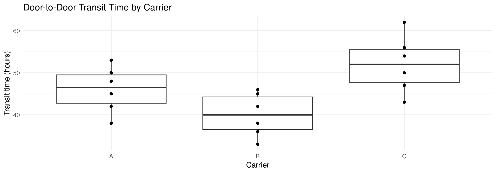
Transit Time by Carrier

A logistics team at a Taiwanese exporter wishes to see if there is a difference in the door-to-door transit time of shipments sent from Taoyuan to a Southeast Asian distribution hub by three carriers. Six recent shipments are randomly selected from each carrier and the transit time is recorded in hours. At \alpha = 0.05, can it be concluded that there is a significant difference in the mean transit times of the three carriers?

Carrier A   Carrier B   Carrier C
    53          46          62
    50          45          56
    48          42          54
    45          38          50
    42          36          47
    38          33          43

(hypothetical data)

Back to Example 12-4

Example 12-2

Solution

Step 1. State the hypotheses and identify the claim.

H_0: \mu_1 = \mu_2 = \mu_3 H_1: \text{At least one mean is different from the others} \ \textit{(claim)}

Step 2. Find the critical value. Since k = 3, N = 18 and \alpha = 0.05,

d.f.N. = k - 1 = 2 \qquad d.f.D. = N - k = 18 - 3 = 15

The critical value is 3.68.

qf(0.95, df1 = 2, df2 = 15)   # Table A-7 rounds this value to 3.68

[1] 3.68232

Example 12-2

Solution

Step 3a-b — the group statistics and the grand mean

carrier_a <- c(53, 50, 48, 45, 42, 38)
carrier_b <- c(46, 45, 42, 38, 36, 33)
carrier_c <- c(62, 56, 54, 50, 47, 43)

mean(carrier_a)

[1] 46

mean(carrier_b)

[1] 40

mean(carrier_c)

[1] 52

var(carrier_a)

[1] 30

var(carrier_b)

[1] 26.8

var(carrier_c)

[1] 46

mean(c(carrier_a, carrier_b, carrier_c))

[1] 46

Example 12-2

Solution

Step 3c-e — the two variance estimates and F

s_B^2 = \frac{6(46-46)^2 + 6(40-46)^2 + 6(52-46)^2}{3-1} = \frac{432}{2} = 216

s_W^2 = \frac{5(30) + 5(26.8) + 5(46)}{5+5+5} = \frac{514}{15} = 34.267

F = \frac{216}{34.267} = 6.304

Steps 4-5. Since 6.304 > 3.68, reject H_0: there is enough evidence that at least one mean differs from the others.

between_var <- (6 * (46 - 46)^2 + 6 * (40 - 46)^2 + 6 * (52 - 46)^2) / (3 - 1)
within_var  <- (5 * 30 + 5 * 26.8 + 5 * 46) / (5 + 5 + 5)

between_var

[1] 216

within_var

[1] 34.26667

between_var / within_var

[1] 6.303502

Example 12-2

Solution

Table 12-3 — Analysis of Variance Summary Table for Example 12-2

Source	Sum of squares	d.f.	Mean square	F
Between groups	432.000	2	216.000	6.304
Within groups (error)	514.000	15	34.267
Total	946.000	17

In Table A-7 the value 6.304 falls between 4.77 (\alpha = 0.025) and 6.36 (\alpha = 0.01), so 0.01 < \text{P-value} < 0.025 and H_0 is rejected.

transit <- data.frame(
  transit_hours = c(carrier_a, carrier_b, carrier_c),
  carrier       = rep(c("A", "B", "C"), each = 6)
)
transit_aov <- aov(transit_hours ~ carrier, data = transit)

summary(transit_aov)

            Df Sum Sq Mean Sq F value Pr(>F)  
carrier      2    432  216.00   6.304 0.0103 *
Residuals   15    514   34.27                 
---
Signif. codes:  0 '***' 0.001 '**' 0.01 '*' 0.05 '.' 0.1 ' ' 1

Example 12-2

Solution

Draw figure — the data behind the test

ggplot(transit, aes(carrier, transit_hours)) +
  geom_boxplot() +
  geom_point() +
  labs(title = "Door-to-Door Transit Time by Carrier",
       x = "Carrier", y = "Transit time (hours)")

After the F Test

Caution

When the null hypothesis is rejected in ANOVA, it only means that at least one mean is different from the others. To locate the difference or differences among the means, it is necessary to use other tests such as the Tukey, the Scheffé or the Bonferroni test.

Section 12-2: The Scheffé Test, Tukey Test, and Bonferroni Test

Locating the Difference

When the null hypothesis is rejected using the F test, the researcher may want to know where the difference among the means is. Several procedures have been developed to determine where the significant differences lie after the ANOVA has been performed. Among the most commonly used are the Scheffé test, the Tukey test and the Bonferroni test.

To conduct the Scheffé test, the means are compared two at a time, using all possible combinations of means. For example, if there are three means, the comparisons are

\bar{X}_1 \text{ versus } \bar{X}_2 \qquad \bar{X}_1 \text{ versus } \bar{X}_3 \qquad \bar{X}_2 \text{ versus } \bar{X}_3

The Scheffé Test

Formula for the Scheffé Test Statistic

F_S = \frac{(\bar{X}_i - \bar{X}_j)^2}{s_W^2 \left[ (1/n_i) + (1/n_j) \right]}

where \bar{X}_i and \bar{X}_j are the means of the samples being compared, n_i and n_j are the respective sample sizes, and s_W^2 is the within-group variance.

To find the critical value F' for the Scheffé test, multiply the critical value for the F test by k - 1:

F' = (k - 1)(C.V.)

There is a significant difference between the two means being compared when F_S > F'.

Example 12-3

Scheffé Test for the Store Revenue Data

Use the Scheffé test to test each pair of means in Example 12-1 to see if a significant difference exists between each pair of means. Use \alpha = 0.05.

Recall \bar{X}_1 = 72 (n_1 = 4), \bar{X}_2 = 65 (n_2 = 5), \bar{X}_3 = 52 (n_3 = 3) and s_W^2 = 56.

Example 12-3

Solution

The F critical value for Example 12-1 is 4.256, which Table A-7 rounds to 4.26. The critical value for the individual tests with d.f.N. = 2 and d.f.D. = 9 is

F' = (k-1)(C.V.) = (3-1)(4.256) = 8.513

a. For \bar{X}_1 versus \bar{X}_2: F_S = \dfrac{(72 - 65)^2}{56 \left( \frac{1}{4} + \frac{1}{5} \right)} = 1.944. Since 1.944 < 8.513, \mu_1 is not significantly different from \mu_2.

b. For \bar{X}_1 versus \bar{X}_3: F_S = \dfrac{(72 - 52)^2}{56 \left( \frac{1}{4} + \frac{1}{3} \right)} = 12.245. Since 12.245 > 8.513, \mu_1 is significantly different from \mu_3.

c. For \bar{X}_2 versus \bar{X}_3: F_S = \dfrac{(65 - 52)^2}{56 \left( \frac{1}{5} + \frac{1}{3} \right)} = 5.658. Since 5.658 < 8.513, \mu_2 is not significantly different from \mu_3.

Hence only the mean revenue of the MRT kiosks differs significantly from the mean revenue of the suburban stores.

Example 12-3

Solution

The same test in R

(72 - 65)^2 / (56 * (1 / 4 + 1 / 5))

[1] 1.944444

(72 - 52)^2 / (56 * (1 / 4 + 1 / 3))

[1] 12.2449

(65 - 52)^2 / (56 * (1 / 5 + 1 / 3))

[1] 5.658482

(3 - 1) * qf(0.95, df1 = 2, df2 = 9)

[1] 8.512989

A Note on the Scheffé Test

Caution

On occasion, when the F test statistic is greater than the critical value, the Scheffé test may not show any significant differences in the pairs of means. This result occurs because the difference may actually lie in the average of two or more means when compared with the other mean. The Scheffé test can be used to make these types of comparisons, but the technique is beyond the scope of this book.

The Tukey Test

The Tukey test can also be used after the analysis of variance has been completed to make pairwise comparisons between means when the groups have the same sample size. The symbol for the test statistic in the Tukey test is q.

Formula for the Tukey Test

q = \frac{\bar{X}_i - \bar{X}_j}{\sqrt{s_W^2 / n}}

where \bar{X}_i and \bar{X}_j are the means of the samples being compared, n is the common sample size, and s_W^2 is the within-group variance.

When the absolute value of q is greater than the critical value for the Tukey test, there is a significant difference between the two means being compared.

The critical value is found in Table A-9, where k is the number of means in the original problem (across the top row) and v = N - k is the degrees of freedom for s_W^2 (in the left column).

Example 12-4

Tukey Test for the Carrier Transit Data

Using the Tukey test, test each pair of means in Example 12-2 to see whether a specific difference exists, at \alpha = 0.05.

Recall \bar{X}_1 = 46 (Carrier A), \bar{X}_2 = 40 (Carrier B), \bar{X}_3 = 52 (Carrier C), s_W^2 = 34.267 and n = 6.

Example 12-4

Solution

a. For \bar{X}_1 versus \bar{X}_2: q = \dfrac{46 - 40}{\sqrt{34.267/6}} = 2.511

b. For \bar{X}_1 versus \bar{X}_3: q = \dfrac{46 - 52}{\sqrt{34.267/6}} = -2.511

c. For \bar{X}_2 versus \bar{X}_3: q = \dfrac{40 - 52}{\sqrt{34.267/6}} = -5.021

Since k = 3, d.f. = 18 - 3 = 15 and \alpha = 0.05, the critical value from Table A-9 is 3.67. The only q value greater in absolute value than the critical value is the one for the difference between \bar{X}_2 and \bar{X}_3. The conclusion is that there is a significant difference in the mean transit times of Carrier B and Carrier C.

Example 12-4

Solution

The same test in R

(46 - 40) / sqrt(34.267 / 6)

[1] 2.510665

(46 - 52) / sqrt(34.267 / 6)

[1] -2.510665

(40 - 52) / sqrt(34.267 / 6)

[1] -5.021331

qtukey(0.95, nmeans = 3, df = 15)   # Table A-9 rounds this value to 3.67

[1] 3.673378

Example 12-4

Solution

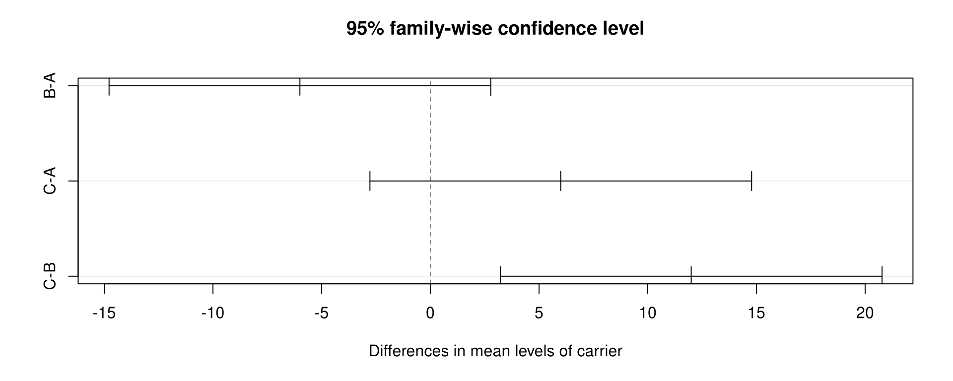
Tukey’s honest significant differences

TukeyHSD(transit_aov)

  Tukey multiple comparisons of means
    95% family-wise confidence level

Fit: aov(formula = transit_hours ~ carrier, data = transit)

$carrier
    diff        lwr       upr     p adj
B-A   -6 -14.778613  2.778613 0.2112790
C-A    6  -2.778613 14.778613 0.2112790
C-B   12   3.221387 20.778613 0.0076917

Only the Carrier C–Carrier B pair has an adjusted P-value below 0.05, which agrees with the hand calculation.

Example 12-4

Solution

Output figure — the family-wise confidence intervals

plot(TukeyHSD(transit_aov))

The Bonferroni Test

The Bonferroni test uses t tests, but the critical value and P-value are adjusted to overcome the problem of the increase in the significance level due to the increase in the number of tests that are being done.

Formula for the Bonferroni Test Statistic

t = \frac{\bar{X}_i - \bar{X}_j}{\sqrt{s_W^2 \left( \dfrac{1}{n_i} + \dfrac{1}{n_j} \right)}} \qquad \text{with } d.f. = N - k

where \bar{X}_i and \bar{X}_j are the means of the samples being compared, n_i and n_j are the respective sample sizes, N is the total number of subjects and k is the number of groups.

The Bonferroni Adjustment

Adjusting the Significance Level and the P-Value

The critical value is adjusted by dividing \alpha by the number of pairings _kC_2 of two sample means. If there are 3 means, _3C_2 = 3 comparisons, so \alpha is divided by 3; if there are 4 means, _4C_2 = 6 comparisons, so \alpha is divided by 6.

For the P-value, multiply the P-value for a single comparison of two means by the number of pairings _kC_2. A P-value can never exceed 1, so any adjusted value larger than 1 is reported as 1.

Example 12-5

Bonferroni Test for the Store Revenue Data

Use the Bonferroni test and \alpha = 0.05 to compare each pair of means in Example 12-1.

Recall \bar{X}_1 = 72 (n_1 = 4), \bar{X}_2 = 65 (n_2 = 5), \bar{X}_3 = 52 (n_3 = 3), s_W^2 = 56, N = 12 and k = 3, so d.f. = 12 - 3 = 9.

Example 12-5

Solution

a. H_0: \mu_1 = \mu_2. \ t = \dfrac{72 - 65}{\sqrt{56 \left( \frac{1}{4} + \frac{1}{5} \right)}} = \dfrac{7}{5.020} = 1.394

The P-value for t = 1.394 with d.f. = 9 is 0.1966. Adjusted: 0.1966 \times 3 = 0.5899. Do not reject H_0.

b. H_0: \mu_1 = \mu_3. \ t = \dfrac{72 - 52}{\sqrt{56 \left( \frac{1}{4} + \frac{1}{3} \right)}} = \dfrac{20}{5.715} = 3.499

The P-value is 0.0067; adjusted 0.0067 \times 3 = 0.0202. Reject H_0 since 0.0202 < 0.05.

c. H_0: \mu_2 = \mu_3. \ t = \dfrac{65 - 52}{\sqrt{56 \left( \frac{1}{5} + \frac{1}{3} \right)}} = \dfrac{13}{5.465} = 2.379

The P-value is 0.0413; adjusted 0.0413 \times 3 = 0.1239, which is not less than \alpha = 0.05. Do not reject H_0.

Example 12-5

Solution

The same test in R

t_stat  <- c((72 - 65) / sqrt(56 * (1 / 4 + 1 / 5)),
             (72 - 52) / sqrt(56 * (1 / 4 + 1 / 3)),
             (65 - 52) / sqrt(56 * (1 / 5 + 1 / 3)))
p_value <- 2 * (1 - pt(t_stat, 9))

t_stat

[1] 1.394433 3.499271 2.378756

p_value

[1] 0.19664741 0.00673123 0.04131181

3 * p_value

[1] 0.58994224 0.02019369 0.12393544

Example 12-5

Solution

Using pairwise.t.test

pairwise.t.test(revenue$daily_revenue, revenue$store_format,
                p.adjust.method = "bonferroni")

    Pairwise comparisons using t tests with pooled SD 

data:  revenue$daily_revenue and revenue$store_format 

         Campus MRT 
MRT      0.59   -   
Suburban 0.12   0.02

P value adjustment method: bonferroni 

The adjusted P-values are 0.59, 0.02 and 0.12 — the same decisions as the hand calculation.

Here P-values are used because the adjusted \alpha would be 0.05 \div 3 = 0.017, and a critical t value for \alpha = 0.017 with 9 d.f. cannot be read from Table A-5.

Which Test Should Be Used?

Choosing Among the Three Tests

• The Scheffé test is the most general. It can be used when the samples are of different sizes, and it can compare, for example, the average of \bar{X}_1 and \bar{X}_2 with \bar{X}_3.
• The Tukey test is more powerful than the Scheffé test for making pairwise comparisons of means, but it requires equal sample sizes.
• A rule of thumb for pairwise comparisons: use the Tukey test when the samples are equal in size and the Scheffé test when the samples differ in size. This rule is followed in this textbook.
• The results of the three tests may differ because of the adjustments made to the critical values and when the test statistics are close to the critical values. There is no common agreement among statisticians as to which test to use; one should use the test that is used in the academic discipline of the research study.

In Example 12-3 and Example 12-5, both the Scheffé test and the Bonferroni test found a difference between \mu_1 and \mu_3.

Section 12-3: Two-Way Analysis of Variance

Two-Way Analysis of Variance

Two-Way ANOVA

The two-way ANOVA is an extension of the one-way analysis of variance; it involves two independent variables. The independent variables are also called factors.

In a study that involves a two-way analysis of variance, the researcher is able to test the effects of two independent variables (or factors) on one dependent variable. In addition, the interaction effect of the two variables can be tested.

The two-way analysis of variance is quite complicated; only a brief introduction is given here.

Treatment Groups

Suppose a researcher wishes to test the effects of two types of plant food (A_1, A_2) and two types of soil (I, II) on plant growth. Other factors, such as water, temperature and sunlight, are held constant. Four groups of plants are set up (Figure 12-4).

Figure 12-4 — Treatment Groups for the Plant Food–Soil Type Experiment

Plant food	Soil type I	Soil type II
A_1	Group 1: food A_1, soil I	Group 2: food A_1, soil II
A_2	Group 3: food A_2, soil I	Group 4: food A_2, soil II

The groups in a two-way ANOVA are called treatment groups. The plants are assigned to the groups at random. This design is called a 2 \times 2 design, since each variable consists of two levels, that is, two different treatments.

Other Two-Way Designs

Figure 12-5 — Some Types of Two-Way ANOVA Designs

Design	Rows (variable A)	Columns (variable B)
3 \times 2	3 levels	2 levels
3 \times 3	3 levels	3 levels
4 \times 3	4 levels	3 levels

There are many different kinds of two-way ANOVA designs, depending on the number of levels of each variable.

The two-way ANOVA lets the researcher test the effects of the plant food and the soil type in a single experiment rather than in separate experiments involving the plant food alone and the soil type alone.

Main Effects and Interaction

Main Effects

The effect of a factor is the change in the response variable that results from changing the level or the type of that factor. These two effects of the independent variables are called the main effects.

Interaction Effect

The interaction effect represents the joint effect of the two factors over and above the effects of each factor considered separately — that is, the types of plant food affect the plant growth differently in different soil types.

When the interaction effect is statistically significant, the researcher should not consider the effects of the individual factors without considering the interaction effect.

The Three Sets of Hypotheses

The two-way ANOVA design has several null hypotheses: one for each independent variable and one for the interaction. For the plant food–soil type problem:

Hypotheses

1. Plant food (factor A).

H_0: There is no difference in means of heights of plants grown using different foods.

H_1: There is a difference in means of heights of plants grown using different foods.

2. Soil type (factor B).

H_0: There is no difference in means of heights of plants grown in different soil types.

H_1: There is a difference in means of heights of plants grown in different soil types.

3. Interaction.

H_0: There is no interaction effect between type of plant food used and type of soil used on plant growth.

H_1: There is an interaction effect between food type and soil type on plant growth.

Table 12-5: Two-Way ANOVA Summary Table

As with the one-way ANOVA, a between-group variance estimate and a within-group variance estimate are calculated, and an F test is performed for each independent variable and for the interaction.

Table 12-5 — ANOVA Summary Table

Source	Sum of squares	d.f.	Mean square	F
Row factor A	SS_A	a-1	MS_A	F_A
Column factor B	SS_B	b-1	MS_B	F_B
Interaction A \times B	SS_{A \times B}	(a-1)(b-1)	MS_{A \times B}	F_{A \times B}
Within (error)	SS_W	ab(n-1)	MS_W
Total	SS_{\text{Total}}	N-1

where a is the number of levels of factor A, b is the number of levels of factor B, and n is the number of subjects in each group.

Formulas for the Two-Way ANOVA

Mean Squares and F Ratios

MS_A = \frac{SS_A}{a-1} \qquad F_A = \frac{MS_A}{MS_W}, \quad d.f.N. = a-1, \ d.f.D. = ab(n-1)

MS_B = \frac{SS_B}{b-1} \qquad F_B = \frac{MS_B}{MS_W}, \quad d.f.N. = b-1, \ d.f.D. = ab(n-1)

MS_{A \times B} = \frac{SS_{A \times B}}{(a-1)(b-1)} \qquad F_{A \times B} = \frac{MS_{A \times B}}{MS_W}, \quad d.f.N. = (a-1)(b-1), \ d.f.D. = ab(n-1)

MS_W = \frac{SS_W}{ab(n-1)}

Assumptions for the Two-Way ANOVA

Assumptions

1. The populations from which the samples were obtained must be normally or approximately normally distributed.
2. The samples must be independent.
3. The variances of the populations from which the samples were selected must be equal.
4. The groups must be equal in sample size.

The assumptions are the same as those for the one-way ANOVA except for sample size — the two-way ANOVA requires equal group sizes. The two-way analysis of variance follows the same five-step hypothesis-testing procedure.

The computational procedure for the sums of squares is quite lengthy; it is omitted in Example 12-6 and only the two-way ANOVA summary table is shown.

Example 12-6

Picking Rate by Method and Shift

An operations manager at a Taoyuan fulfilment centre wishes to see whether the picking method used and the shift worked have any effect on picking productivity. Two picking methods, handheld scanner and voice picking, will be used, and two shifts, day and night, will be used with each method. There will be two pickers in each group, for a total of eight pickers. The number of cartons picked per hour is recorded. Using a two-way analysis of variance, determine if there is an interactive effect, an effect due to the picking method, and an effect due to the shift. Use \alpha = 0.05.

Method        Day shift   Night shift
Scanner          26.6         29.7
                 25.4         28.3
Voice            33.1         25.7
                 31.9         24.3

(hypothetical data)

Example 12-6

Solution

Table 12-6 — ANOVA Summary Table for Example 12-6

Source	Sum of squares	d.f.	Mean square	F
Method (A)	3.125
Shift (B)	10.125
Interaction (A \times B)	55.125
Within (error)	3.400
Total	71.775

Step 1. State the hypotheses.

Picking methods. H_0: There is no difference between the means of the picking rates for the two methods. H_1: There is a difference.

Shifts worked. H_0: There is no difference between the means of the picking rates for the day shift and the night shift. H_1: There is a difference.

Interaction. H_0: There is no interaction effect between the picking method used and the shift worked on the picking rate. H_1: There is an interaction effect.

Example 12-6

Solution

Step 2 — find the critical values for each F test

Each factor has two levels, so a = 2, b = 2 and n = 2.

\text{Factor A: } d.f.N. = a-1 = 1 \qquad \text{Factor B: } d.f.N. = b-1 = 1 \text{Interaction: } d.f.N. = (a-1)(b-1) = 1 \qquad \text{Within (error): } d.f.D. = ab(n-1) = 2 \cdot 2(2-1) = 4

With \alpha = 0.05, d.f.N. = 1 and d.f.D. = 4, all three critical values are 7.71.

qf(0.95, df1 = 1, df2 = 4)   # Table A-7 rounds this value to 7.71

[1] 7.708647

Note. If the factors have different numbers of levels, the critical values will not all be the same. For a factor A with 3 levels and a factor B with 4 levels and 2 subjects per group, d.f.N. = 2, 3 and 6 respectively and d.f.D. = 3 \cdot 4(2-1) = 12.

Example 12-6

Solution

Step 3 — complete the summary table

MS_A = \frac{3.125}{2-1} = 3.125 \qquad MS_B = \frac{10.125}{2-1} = 10.125 MS_{A \times B} = \frac{55.125}{(2-1)(2-1)} = 55.125 \qquad MS_W = \frac{3.400}{4} = 0.850

F_A = \frac{3.125}{0.850} = 3.676 \qquad F_B = \frac{10.125}{0.850} = 11.912 \qquad F_{A \times B} = \frac{55.125}{0.850} = 64.853

Example 12-6

Solution

Table 12-7 — ANOVA Summary Table for Example 12-6

Source	Sum of squares	d.f.	Mean square	F
Method (A)	3.125	1	3.125	3.676
Shift (B)	10.125	1	10.125	11.912
Interaction (A \times B)	55.125	1	55.125	64.853
Within (error)	3.400	4	0.850
Total	71.775	7

Step 4. Make the decision. Since F_B = 11.912 and F_{A \times B} = 64.853 are greater than the critical value 7.71, the null hypotheses concerning the shift worked and the interaction effect should be rejected; F_A = 3.676 is smaller than 7.71, so the null hypothesis for the picking method is not rejected. Since the interaction effect is statistically significant, no decision should be made about the shift effect without further investigation.

Step 5. Summarize the results. Since the null hypothesis for the interaction effect was rejected, it can be concluded that the combination of picking method and shift does affect the picking rate.

Example 12-6

Solution

The same analysis in R

picking <- data.frame(
  cartons_per_hour = c(26.6, 25.4, 29.7, 28.3, 33.1, 31.9, 25.7, 24.3),
  method = rep(c("Scanner", "Voice"), each = 4),
  shift  = rep(c("Day", "Day", "Night", "Night"), times = 2)
)

summary(aov(cartons_per_hour ~ method * shift, data = picking))

             Df Sum Sq Mean Sq F value  Pr(>F)   
method        1   3.13    3.13   3.676 0.12765   
shift         1  10.12   10.12  11.912 0.02602 * 
method:shift  1  55.13   55.13  64.853 0.00129 **
Residuals     4   3.40    0.85                   
---
Signif. codes:  0 '***' 0.001 '**' 0.01 '*' 0.05 '.' 0.1 ' ' 1

Example 12-6

Solution

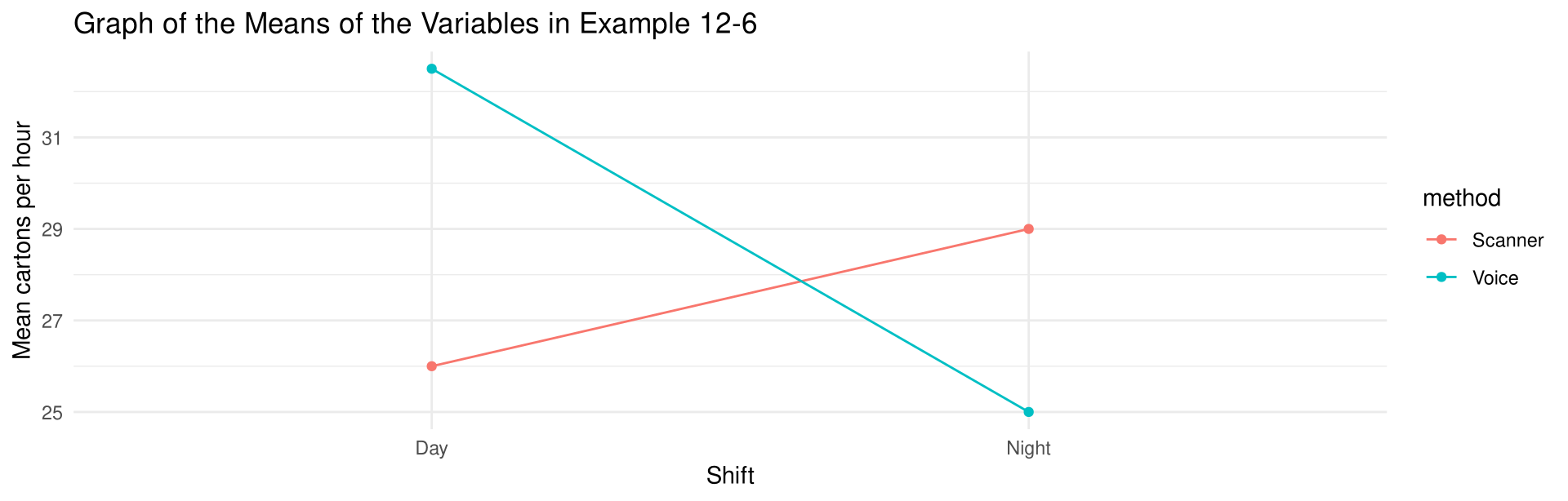
Prepare data — the cell means

Each cell mean is the average of the two pickers assigned to that treatment group.

cell_means <- aggregate(cartons_per_hour ~ method + shift,
                        data = picking, FUN = mean)
cell_means

   method shift cartons_per_hour
1 Scanner   Day             26.0
2   Voice   Day             32.5
3 Scanner Night             29.0
4   Voice Night             25.0

Example 12-6

Solution

Output figure — Figure 12-6, the graph of the means

ggplot(cell_means, aes(shift, cartons_per_hour,
                       color = method, group = method)) +
  geom_line() +
  geom_point() +
  labs(title = "Graph of the Means of the Variables in Example 12-6",
       x = "Shift", y = "Mean cartons per hour")

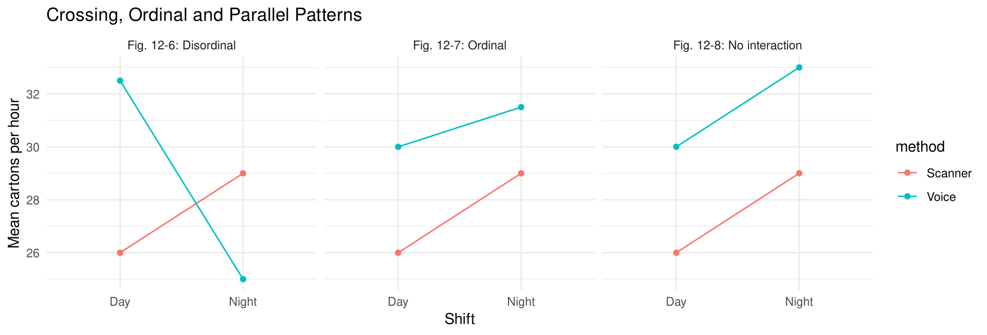
The lines cross, so the interaction is a disordinal interaction.

Interpreting the Interaction

To interpret the results of a two-way analysis of variance, researchers suggest drawing a graph, plotting the means of each group, analyzing the graph, and interpreting the results.

Rules for Reading an Interaction Plot

Pattern of the lines	Interaction	How to interpret the main effects
Lines cross each other and the interaction F is significant	Disordinal interaction (Figure 12-6)	Do not interpret the main effects without considering the interaction effect
Lines do not cross and are not parallel, interaction F significant	Ordinal interaction (Figure 12-7)	The main effects can be interpreted independently of each other
Lines are parallel or approximately parallel, interaction F not significant	No interaction (Figure 12-8)	The main effects can be interpreted independently

If there is no significant interaction effect, the main effects can be interpreted independently; however, if there is a significant interaction effect, the main effects must be interpreted cautiously, if at all.

Interaction Patterns in R

Prepare data — the three patterns of Figures 12-6, 12-7 and 12-8

patterns <- data.frame(
  pattern   = rep(c("Fig. 12-6: Disordinal", "Fig. 12-7: Ordinal",
                    "Fig. 12-8: No interaction"), each = 4),
  method    = rep(c("Scanner", "Scanner", "Voice", "Voice"), times = 3),
  shift     = rep(c("Day", "Night"), times = 6),
  mean_rate = c(26.0, 29.0, 32.5, 25.0,
                26.0, 29.0, 30.0, 31.5,
                26.0, 29.0, 30.0, 33.0)
)

Interaction Patterns in R

Output figure

ggplot(patterns, aes(shift, mean_rate, color = method, group = method)) +
  geom_line() +
  geom_point() +
  facet_wrap(~ pattern) +
  labs(title = "Crossing, Ordinal and Parallel Patterns",
       x = "Shift", y = "Mean cartons per hour")

Beyond a 2 \times 2 Design

Caution

Example 12-6 was a 2 \times 2 two-way analysis of variance, since each independent variable had two levels. For other designs, such as a 3 \times 2 or a 4 \times 3 ANOVA, interpretation of the results can be quite complicated. Procedures using tests such as the Tukey and Scheffé tests for analyzing the cell means exist and are similar to the tests shown for the one-way ANOVA, but they are beyond the scope of this textbook. Many other designs, such as three-factor designs and repeated-measure designs, are also beyond the scope of this book.

Important Terms

Chapter 12 Vocabulary

analysis of variance (ANOVA) · ANOVA summary table · between-group variance · Bonferroni test · disordinal interaction · factors · interaction effect · level · main effects · mean square · one-way ANOVA · ordinal interaction · Scheffé test · sum of squares between groups · sum of squares within groups · treatment groups · Tukey test · two-way ANOVA · within-group variance

Key Formulas

Formulas for the ANOVA Test

\bar{X}_{GM} = \frac{\sum X}{N} \qquad F = \frac{s_B^2}{s_W^2}

s_B^2 = \frac{\sum n_i (\bar{X}_i - \bar{X}_{GM})^2}{k-1} \qquad s_W^2 = \frac{\sum (n_i - 1)s_i^2}{\sum (n_i - 1)}

d.f.N. = k - 1 \qquad d.f.D. = N - k \qquad N = n_1 + n_2 + \cdots + n_k

Key Formulas

Formulas for the Scheffé, Tukey and Bonferroni Tests

F_S = \frac{(\bar{X}_i - \bar{X}_j)^2}{s_W^2 \left[ (1/n_i) + (1/n_j) \right]} \qquad \text{and} \qquad F' = (k-1)(C.V.)

q = \frac{\bar{X}_i - \bar{X}_j}{\sqrt{s_W^2 / n}}, \qquad d.f.N. = k \ \text{ and } \ d.f.D. = \text{degrees of freedom for } s_W^2

t = \frac{\bar{X}_i - \bar{X}_j}{\sqrt{s_W^2 \left( \dfrac{1}{n_i} + \dfrac{1}{n_j} \right)}} \qquad \text{with } d.f. = N - k

Key Formulas

Formulas for the Two-Way ANOVA

MS_A = \frac{SS_A}{a-1} \qquad F_A = \frac{MS_A}{MS_W} \qquad d.f.N. = a-1, \ d.f.D. = ab(n-1)

MS_B = \frac{SS_B}{b-1} \qquad F_B = \frac{MS_B}{MS_W} \qquad d.f.N. = b-1, \ d.f.D. = ab(n-1)

MS_{A \times B} = \frac{SS_{A \times B}}{(a-1)(b-1)} \qquad F_{A \times B} = \frac{MS_{A \times B}}{MS_W} \qquad d.f.N. = (a-1)(b-1)

MS_W = \frac{SS_W}{ab(n-1)}

Key Takeaways

1. The F test can compare three or more means; the technique is called the analysis of variance (ANOVA). Multiple t tests are not used because they ignore the other means, inflate the type I error rate, and grow rapidly in number.
2. ANOVA uses two estimates of the population variance: the between-group variance s_B^2 (the variance of the sample means) and the within-group variance s_W^2 (the overall variance of all the values). The test statistic is F = s_B^2 / s_W^2, with d.f.N. = k-1 and d.f.D. = N-k, and the test is always right-tailed.
3. When there is no significant difference among the means, the two estimates are approximately equal and F is close to 1; when a difference exists, s_B^2 is much larger and F is significant.

Key Takeaways

4. A significant F says only that at least one mean differs; the Scheffé, Tukey and Bonferroni tests locate the difference. Use Tukey when the sample sizes are equal and Scheffé when they differ; the Scheffé critical value is F' = (k-1)(C.V.) and the Bonferroni P-value is multiplied by _kC_2.
5. The two-way ANOVA tests the effects of two independent variables and their interaction on one dependent variable, and requires equal group sizes.
6. If the interaction is significant and the lines in the interaction plot cross, the interaction is disordinal and the main effects must not be interpreted on their own; if the lines do not cross, the interaction is ordinal and the main effects may be interpreted independently; parallel lines indicate no interaction.

Acknowledgement

• Copyright notice. These teaching materials follow the organization and terminology of Bluman, A. G. (2023). Elementary statistics: A step by step approach (11th ed.). McGraw Hill. All rights in the original work are reserved by its authors and publishers.

• Original examples. Every worked example, data set, and R script in these slides was written for this course. The data are hypothetical unless stated otherwise.

• Non-commercial use only. These materials are strictly intended for educational purposes and must not be used for commercial gain or profit.

• Proper attribution. Any reproduction, distribution, or use of these materials must provide proper attribution to the original source.