Statistics

Chapter 14: Sampling and Simulation

Yu-You Liou

Shih Chien University

2026-10-08

Overview

Chapter 14 covers how researchers sample, how surveys bias results, simulation with random numbers, and big data.

Section	Topics
14-1	Why sample; unbiased vs. biased samples; four kinds of bias; the four basic sampling methods and others
14-2	Survey types; five faulty-question mistakes; other sources of response bias; open- vs. closed-ended items
14-3	Simulation; the Monte Carlo method in five steps; random numbers
14-4	Big data; the 3 V’s and variability; structured vs. unstructured data

Chapter Objectives

After completing this chapter, you should be able to

1. Demonstrate a knowledge of the four basic sampling methods.
2. Recognize faulty questions on a survey and other factors that can bias responses.
3. Solve problems, using simulation techniques.
4. Explain the basic concepts of big data.

Introduction

Pollsters such as Gallup and Nielsen, and the U.S. Census Bureau, gather information by selecting samples from well-defined populations. As in Chapter 1, the subjects in the sample are a subgroup of the subjects in the population, and the sampling methods used to choose them rely on random numbers.

• Since many statistical studies use surveys and questionnaires, Section 14-2 looks at how those instruments can go wrong.
• Random numbers are also used in simulation: instead of studying a real-life situation that may be costly or dangerous, researchers create a similar situation in a laboratory or on a computer and study that instead.
• Section 14-4 introduces big data, the very large, fast-growing and highly varied data sets that computers now make it possible to collect and analyze.

Section 14-1: Common Sampling Techniques

Populations, Samples and Randomness

In Chapter 1 a population was defined as all subjects (human or otherwise) under study. Since some populations are very large, researchers cannot use every single subject, so a sample must be selected. Technically any subgroup of the population can be called a sample, but for researchers to make valid inferences about population characteristics, the sample must be random.

Random Sample

For a sample to be a random sample, every member of the population must have an equal chance of being selected.

Unbiased and Biased Samples

Unbiased Sample and Biased Sample

When a sample is chosen at random from a population, it is said to be an unbiased sample — the sample is, for the most part, representative of the population.

If a sample is selected incorrectly, it may be a biased sample. Samples are biased when some type of systematic error has been made in the selection of the subjects.

Four Types of Biased Samples

Ways a Sample Can Become Biased

Type of bias	When it occurs
Sampling or selection bias	Some subjects are more likely to be included in the survey or study than others
Nonresponse bias	Subjects who do not respond to a survey question would answer it differently than those who do respond
Response or interviewer bias	The subject gives a different response than the respondent truly believes
Volunteer bias	Volunteers are used, and they may be more interested in the survey or study and so answer or participate differently than randomly selected subjects

Why a Sample Is Used

Three Reasons for Sampling

1. It saves the researcher time and money.
2. It enables the researcher to get information that might not be obtainable otherwise. A researcher cannot analyze every drop of a person’s blood for cholesterol without killing the person, and a company cannot test every cable to destruction, since it would then have no cables left to sell.
3. It enables the researcher to get more detailed information about a particular subject. With only a few people surveyed, in-depth interviews are possible.

This does not mean that the smaller the sample, the better — the opposite is true. In general, larger samples, if correct sampling techniques are used, give more reliable information about the population.

A Representative Sample

It would be ideal if the sample were a perfect miniature of the population in all characteristics. This ideal is impossible to achieve, because there are so many human traits (height, weight, IQ, and so on). The best that can be done is to select a sample that is representative with respect to some characteristics, preferably those pertaining to the study.

For example, if one-half of the population subjects are female, then approximately one-half of the sample subjects should be female. Likewise, other characteristics such as age, socioeconomic status and IQ should be represented proportionately.

To obtain unbiased samples, statisticians have developed several basic sampling methods. The most common are random, systematic, stratified and cluster sampling.

Random Sampling

A random sample is obtained by using methods such as random numbers, which can be generated from calculators, computers or tables. In random sampling the basic requirement is that, for a sample of size n, all possible samples of this size have an equal chance of being selected from the population.

Caution

Three commonly used methods are not random sampling, because not all possible samples of a specific size have an equal chance of being selected:

1. Asking “the person on the street” — many people are at home or at work while the interview is conducted and so have no chance of being selected.
2. Asking a question on radio or television and having listeners or viewers call in — only those who feel strongly may respond, and many never heard or saw the program.
3. Asking people to respond by mail or email — only those who are concerned and who have the time are likely to respond.

Two Correct Methods

How to Select a Random Sample

Method 1. Number each element of the population, place the numbers on cards, put the cards in a hat or fishbowl, mix them, and select the sample by drawing the cards. The numbers must be well mixed; on occasion the numbers chosen turn out to be those that were placed in the bowl last.

Method 2 (preferred). Use a table of random numbers, such as Table A-1 in Appendix A, or numbers generated by a computer.

Random samples can be selected with or without replacement. If the same member of the population cannot be used more than once in the study, the sample is selected without replacement — once a random number is selected, it cannot be used again.

Table 14-1: Part of Table A-1, the Table of Random Numbers

60035  97320  62543  61404  94367  07080  66112  56180  15813  15978
64072  76075  91393  88948  99244  60809  10784  36380  05721  24481
14914  85608  96871  74743  73692  53664  67727  21440  13326  98590
93723  60571  17559  96844  88678  89256  75120  62384  77414  24023
86656  43736  62752  53819  81674  43490  07850  61439  52300  55063
31286  27544  44129  51107  53727  65479  09688  57355  20426  44527
95519  78485  20269  64027  53229  59060  99269  12140  97864  31064
78019  75498  79017  22157  22893  88109  57998  02582  34259  11405
45487  22433  62809  98924  96769  24955  60283  16837  02070  22051
64769  25684  33490  25168  34405  58272  90124  92954  43663  39556

The theory behind random numbers is that each digit, 0 through 9, has an equal probability of occurring: in every sequence of 10 digits, each digit has a probability of \dfrac{1}{10} of occurring. This does not mean that every sequence of 10 digits contains each digit. It means that on average each digit will occur once — the digit 2 may occur 3 times in one sequence of 10 digits and not at all in later ones, averaging to a probability of \dfrac{1}{10}.

Generating Random Numbers in R

set.seed(2023)
sample(0:9, size = 50, replace = TRUE)

 [1] 4 8 7 2 9 1 0 0 0 0 4 7 1 2 3 4 7 8 6 8 1 5 4 8 1 6 6 0 4 0 5 3 5 5 1 1 2 7
[39] 3 7 6 0 9 3 0 4 9 2 0 9

sample(1:50, size = 10)

 [1] 15 21 12 48 31 28 43  9 22 27

Each digit 0 through 9 is equally likely, so the first call reproduces the behaviour of the random-number table. The second call draws ten numbers between 1 and 50 without replacement, which is what sample() does by default.

Example 14-1

Auditing Convenience-Store Branches

A convenience-store chain operates 50 branches in northern Taiwan and wants to send mystery shoppers to some of them. The audit budget covers only 10 branches, and head office wants them chosen at random so that no district manager can predict who will be visited. Select a random sample of 10 branches from the 50. (hypothetical data)

Note: This answer is not unique.

Back to Example 14-2

Example 14-1

Solution

Step 1. Number each branch from 1 to 50. Here the branches are numbered alphabetically by the district they serve.

01. Bade         14. Luzhou       27. Shilin       40. Wulai
02. Bali         15. Luzhu        28. Shimen       41. Xindian
03. Banqiao      16. Nangang      29. Shuangxi     42. Xinyi
04. Beitou       17. Neihu        30. Shulin       43. Xinzhuang
05. Daan         18. Pinglin      31. Songshan     44. Xizhi
06. Datong       19. Pingxi       32. Taishan      45. Yangmei
07. Daxi         20. Pingzhen     33. Tamsui       46. Yingge
08. Gongliao     21. Ruifang      34. Taoyuan      47. Yonghe
09. Guishan      22. Sanchong     35. Tucheng      48. Zhonghe
10. Jinshan      23. Sanxia       36. Wanhua       49. Zhongli
11. Keelung      24. Sanzhi       37. Wanli        50. Zhongshan
12. Linkou       25. Shenkeng     38. Wenshan
13. Longtan      26. Shiding      39. Wugu

Example 14-1

Solution

Step 2. Using the table of random numbers, find a starting point. Close your eyes and place your finger anywhere on the table. Here the finger lands on 62543, the first number in the third column. Use the last two digits, 4 and 3, so the first random number is 43.

Continue down the column. The next number is 91393, but 93 is beyond 1 through 50, so skip it. Keep going until the column ends, then start at the top of the next column. If the same number appears twice, skip it: 74743 gives 43 again, which is already in the sample.

The ten random numbers are 43,\ 29,\ 17,\ 09,\ 04,\ 48,\ 44,\ 19,\ 07,\ 27

Example 14-1

Solution

Step 3. These correspond to the following branches, which the mystery shoppers will visit:

Number	Branch	Number	Branch
43	Xinzhuang	48	Zhonghe
29	Shuangxi	44	Xizhi
17	Neihu	19	Pingxi
09	Guishan	07	Daxi
04	Beitou	27	Shilin

Example 14-1

Solution

Same selection in R

branches <- c(
  "Bade","Bali","Banqiao","Beitou","Daan","Datong","Daxi","Gongliao","Guishan","Jinshan",
  "Keelung","Linkou","Longtan","Luzhou","Luzhu","Nangang","Neihu","Pinglin","Pingxi","Pingzhen",
  "Ruifang","Sanchong","Sanxia","Sanzhi","Shenkeng","Shiding","Shilin","Shimen","Shuangxi","Shulin",
  "Songshan","Taishan","Tamsui","Taoyuan","Tucheng","Wanhua","Wanli","Wenshan","Wugu","Wulai",
  "Xindian","Xinyi","Xinzhuang","Xizhi","Yangmei","Yingge","Yonghe","Zhonghe","Zhongli","Zhongshan")

branches[c(43, 29, 17, 9, 4, 48, 44, 19, 7, 27)]

 [1] "Xinzhuang" "Shuangxi"  "Neihu"     "Guishan"   "Beitou"    "Zhonghe"  
 [7] "Xizhi"     "Pingxi"    "Daxi"      "Shilin"   

Example 14-1

Solution

A fresh random sample

set.seed(1114)
audit_numbers <- sort(sample(1:50, size = 10))

audit_numbers

 [1]  9 10 11 20 24 33 36 40 43 48

branches[audit_numbers]

 [1] "Guishan"   "Jinshan"   "Keelung"   "Pingzhen"  "Sanzhi"    "Tamsui"   
 [7] "Wanhua"    "Wulai"     "Xinzhuang" "Zhonghe"  

sample() draws without replacement; both samples are correct.

Limitation of Random Sampling

Caution

Random sampling has one limitation. If the population is extremely large, it is time-consuming to number and select the sample elements.

Systematic Sampling

Systematic Sample

A systematic sample is a sample obtained by numbering each element in the population, selecting some random starting point, and then selecting every kth element (third or fifth or tenth, and so on) from the population to be included in the sample.

Example 14-2

A Systematic Audit Schedule

Using the population of 50 branches in Example 14-1, select a systematic sample of 10 branches.

Example 14-2

Solution

Step 1. Number the population units as shown in Example 14-1.

Step 2. Since there are 50 branches and 10 are to be selected, the rule is to select every fifth branch. This rule was determined by dividing 50 by 10, which yields 5.

Step 3. Using the table of random numbers, select the first number (from 1 to 5) at random. In this case 2 was selected.

Step 4. Select every fifth number starting with 2.

2,\ 7,\ 12,\ 17,\ 22,\ 27,\ 32,\ 37,\ 42,\ 47

Example 14-2

Solution

The branches selected are:

Number	Branch	Number	Branch
2	Bali	27	Shilin
7	Daxi	32	Taishan
12	Linkou	37	Wanli
17	Neihu	42	Xinyi
22	Sanchong	47	Yonghe

Example 14-2

Solution

Same selection in R

set.seed(2024)
random_start   <- sample(1:5, size = 1)
audit_schedule <- seq(random_start, 50, by = 5)

audit_schedule

 [1]  2  7 12 17 22 27 32 37 42 47

branches[audit_schedule]

 [1] "Bali"     "Daxi"     "Linkou"   "Neihu"    "Sanchong" "Shilin"  
 [7] "Taishan"  "Wanli"    "Xinyi"    "Yonghe"  

Advantages and Cautions of Systematic Sampling

The advantage of systematic sampling is the ease of selecting the sample elements. In many cases a numbered list of the population units already exists, such as a factory manager’s list of employees or an in-house telephone directory.

Caution

You must be careful how the items are arranged on the list.

• If the list runs 1. Husband, 2. Wife, 3. Husband, 4. Wife, then the starting number could produce a sample of all males or all females, depending on whether the starting number and the number added are even or odd.
• If the list were arranged in order of the heights of individuals, two samples would give very different averages depending on whether the starting number was small or large.

Stratified Sampling

Stratified Sample

A stratified sample is a sample obtained by dividing the population into subgroups, called strata, according to various homogeneous (similar) characteristics and then randomly selecting members from each stratum for the sample.

For example, a population may consist of males and females who are smokers or nonsmokers. The researcher divides the population into four subgroups — male smokers, male nonsmokers, female smokers, female nonsmokers — and then selects a random sample from each subgroup. This ensures the sample is representative on the basis of gender and smoking, although it may not be representative on the basis of other characteristics.

Example 14-3

Selecting Member Companies

An exporters’ association has the 20 member companies listed below, each classified by industry (electronics or food) and by firm size (small or large). Select a sample of eight companies on the basis of industry and size by stratification. (hypothetical data)

 1. Aurora Tech       E  S    11. Helios Optics      E  L
 2. Harvest Sauce     F  L    12. Ruby Fruit         F  L
 3. Camellia Tea      F  S    13. Orchid Circuits    E  S
 4. Beacon Semi       E  L    14. Pomelo Foods       F  S
 5. Jade Snack        F  S    15. Granite Boards     E  L
 6. Kingfisher Micro  E  S    16. Silver Carp Foods  F  L
 7. Skyline Vision    E  L    17. Zenith Modules     E  S
 8. Golden Grain      F  L    18. Willow Bakery      F  S
 9. Lotus Noodle      F  S    19. Summit Cable       E  L
10. Nimbus Devices    E  S    20. Teal Bean Foods    F  L

E = electronics, F = food; S = small, L = large.

Example 14-3

Solution

Step 1. Divide the population into two subgroups, electronics firms and food firms.

Step 2. Divide each subgroup further into small firms and large firms.

Group 1 (E, S)              Group 2 (E, L)
1. Aurora Tech              1. Beacon Semi
2. Kingfisher Micro         2. Skyline Vision
3. Nimbus Devices           3. Helios Optics
4. Orchid Circuits          4. Granite Boards
5. Zenith Modules           5. Summit Cable

Group 3 (F, S)              Group 4 (F, L)
1. Camellia Tea             1. Harvest Sauce
2. Jade Snack               2. Golden Grain
3. Lotus Noodle             3. Ruby Fruit
4. Pomelo Foods             4. Silver Carp Foods
5. Willow Bakery            5. Teal Bean Foods

Example 14-3

Solution

Step 3. Determine how many companies to select from each subgroup for proportional representation. There are four groups, and a total of eight companies is needed, so two companies must be selected from each subgroup.

Step 4. Select two companies from each group by using random numbers. In this case the random numbers are

Group 1	Group 2	Group 3	Group 4
Companies 4 and 3	Companies 4 and 2	Companies 5 and 3	Companies 2 and 3

The stratified sample then consists of the following companies:

Orchid Circuits	Granite Boards
Nimbus Devices	Skyline Vision
Willow Bakery	Golden Grain
Lotus Noodle	Ruby Fruit

Example 14-3

Solution

Prepare data

members <- data.frame(
  company  = c("Aurora Tech","Harvest Sauce","Camellia Tea","Beacon Semi","Jade Snack",
               "Kingfisher Micro","Skyline Vision","Golden Grain","Lotus Noodle","Nimbus Devices",
               "Helios Optics","Ruby Fruit","Orchid Circuits","Pomelo Foods","Granite Boards",
               "Silver Carp Foods","Zenith Modules","Willow Bakery","Summit Cable","Teal Bean Foods"),
  industry = c("Electronics","Food","Food","Electronics","Food",
               "Electronics","Electronics","Food","Food","Electronics",
               "Electronics","Food","Electronics","Food","Electronics",
               "Food","Electronics","Food","Electronics","Food"),
  size     = c("Small","Large","Small","Large","Small",
               "Small","Large","Large","Small","Small",
               "Large","Large","Small","Small","Large",
               "Large","Small","Small","Large","Large")
)
table(members$industry, members$size)

             
              Large Small
  Electronics     5     5
  Food            5     5

Example 14-3

Solution

Draw two companies from each stratum

set.seed(1403)
strata <- group_by(members, industry, size)

slice_sample(strata, n = 2)

# A tibble: 8 × 3
# Groups:   industry, size [4]
  company         industry    size 
  <chr>           <chr>       <chr>
1 Granite Boards  Electronics Large
2 Skyline Vision  Electronics Large
3 Orchid Circuits Electronics Small
4 Nimbus Devices  Electronics Small
5 Golden Grain    Food        Large
6 Ruby Fruit      Food        Large
7 Willow Bakery   Food        Small
8 Lotus Noodle    Food        Small

Each of the four strata contributes exactly two companies, so both industries and both size classes are represented.

Advantages and Drawbacks of Stratification

Stratified Sampling

Major advantage. It ensures representation of all population subgroups that are important to the study.

Two major drawbacks.

1. If there are many variables of interest, dividing a large population into representative subgroups requires a great deal of effort.
2. If the variables are somewhat complex or ambiguous, such as beliefs, attitudes or prejudices, it is difficult to separate individuals into subgroups according to those variables.

Cluster Sampling

Cluster Sample

A cluster sample is a sample obtained by selecting a preexisting or natural group, called a cluster, and using the members in the cluster for the sample.

Many studies in education use already existing classes, such as the seventh grade in Wilson Junior High School. The voters of an electoral district might be surveyed about a mayoral candidate, or the residents of an entire city block polled about household incomes. Researchers may use all units of a cluster if that is feasible, or select only part of a cluster by random methods.

Advantages and Disadvantage of Cluster Sampling

Cluster Sampling

Three advantages. A cluster sample (1) can reduce costs, (2) can simplify fieldwork, and (3) is convenient. In a dental study X-raying fourth-grade students’ teeth, it is simple to select a single classroom and bring the X-ray equipment to the school; other methods might require transporting the machine to several schools or the pupils to the dental office.

Major disadvantage. The elements in a cluster may not have the same variations in characteristics as elements selected individually from a population, because people in specific clusters such as neighborhoods or clubs tend to be more homogeneous — similar incomes, similar cars, similar houses and, for the most part, similar habits.

Other Types of Sampling Techniques

Four Additional Methods

Sequence sampling, used in quality control, samples successive units taken from production lines to ensure that the products meet certain standards set by the manufacturing company.

Double sampling gives a very large population a questionnaire to determine those who meet the qualifications for a study. After the questionnaires are reviewed, a second, smaller population is defined, and a sample is selected from this group.

Multistage sampling uses a combination of sampling methods.

Convenience sampling selects subjects from the population who are available to use. These samples are usually not representative of the population, and their use can lead to biased conclusions.

A Multistage Example

Suppose a research organization wants to conduct a nationwide survey for a new product being manufactured. A sample can be obtained by using the following combination of methods.

1. Divide the 50 states into four or five regions (or clusters).
2. Select several states from each region at random.
3. Divide the states into areas by using large cities and small towns, and select samples of these areas.
4. Divide each city and each town into districts or wards.
5. Select streets in these wards at random, and give the families living on these streets samples of the product to test and report on.

This hypothetical example illustrates a typical multistage sampling method.

Procedure Table: Conducting a Sample Survey

Nine Steps

Step	Action
1	Decide what information is needed.
2	Determine how the data will be collected (phone interview, mail survey, and so on).
3	Select the information-gathering instrument or design the questionnaire if one is not available.
4	Set up a sampling list, if possible.
5	Select the best method for obtaining the sample (random, systematic, stratified, cluster or other).
6	Conduct the survey and collect the data.
7	Tabulate the data.
8	Conduct the statistical analysis.
9	Report the results.

How Large a Sample Do I Need?

The answer is based on several things. Two important considerations are time and money: the more of both a researcher has, the larger the sample can be. When random samples are used, larger samples can result in more reliable conclusions.

Also, as shown in Chapter 7, an actual sample size can be computed if the researcher knows the confidence level and the degree of accuracy (the margin of error) desired.

Section 14-2: Surveys and Questionnaire Design

What Is a Survey?

A survey is conducted when a sample of individuals is asked to respond to questions about a particular subject.

Two Types of Surveys

Interviewer-administered surveys require a person to ask the questions. The interview can be conducted face to face in an office, on a street, or in the mall, or via telephone.

Self-administered surveys can be done by mail, email, the Internet, or in a group setting such as a classroom.

Wording Changes the Answer

When analyzing the results of surveys you should be very careful about the interpretations, because the way a question is phrased can influence the way people respond.

Question asked	In favor	Against
Do you favor a small charge on single-use shopping bags, to cut plastic waste in the city?	78%	18%
Should shoppers be made to pay a new fee on every bag issued at a convenience store?	34%	59%

Both questions ask about the same policy, yet the responses are almost reversed: the first names the purpose of the charge, the second names only its cost. Different phrasings of one question produce different answers. (hypothetical data)

Five Common Mistakes in Writing Questions

Avoid These Mistakes

1. Asking biased questions. “Are you going to vote for candidate Jones even though the latest survey indicates that he will lose the election?” may dissuade some people from answering in the affirmative, compared with “Are you going to vote for candidate Jones?”
2. Using confusing words. “Do you think people would live longer if they were on a diet?” can be misinterpreted, since there are weight-loss diets, low-salt diets, medically prescribed diets, and so on.
3. Asking double-barreled questions. “Are you in favor of a special tax to provide national health care for the citizens of the United States?” really asks two questions at once.
4. Using double negatives in questions. “Do you feel that it is not appropriate to have areas where people cannot smoke?” is very confusing since not is used twice.
5. Ordering questions improperly. Asking “At what age should an elderly person not be permitted to drive?” before asking respondents to list problems of elderly people leads them to answer transportation.

Other Factors That Bias a Survey

Caution

• Answering about an unknown subject. A participant may know nothing about the subject but answer anyway to avoid being considered uninformed. Many people would answer yes or no to “Would you be in favor of giving pensions to the widows of unknown soldiers?”, a question that makes no sense.
• Telling the interviewer what they want to hear. Asked “How often do you lie?”, people understate the incidences of their lying.
• Known identity. Participants respond differently depending on whether their identity is known, especially on sensitive issues such as income, sexuality and abortion. Researchers try to ensure confidentiality (keeping the respondent’s identity secret) rather than anonymity (soliciting unsigned responses); many people are suspicious in either case.
• Time and place. A survey on airline safety conducted immediately after a major crash may give very different results from one taken in a year with no major disasters.

Open-Ended and Closed-Ended Questions

Two Types of Questions

An open-ended question is one such as “List three activities that you plan to spend more time on when you retire.”

A closed-ended question is one such as “Which one of these activities do you plan to spend more time on after you retire: traveling; eating out; fishing and hunting; exercising; visiting relatives?”

The trade-off. With a closed-ended question, respondents are forced to choose the answers the researcher gives and cannot supply their own. With an open-ended question, the results may be so varied that summarizing them is difficult, if not impossible.

Designing and Using a Questionnaire

Good Practice

• Conduct a pilot study to test the design and usage of the questionnaire, that is, its validity. The pilot study helps the researcher to pretest the questionnaire to see whether it meets the objectives of the study, and to rewrite any questions that are misleading or ambiguous.
• If the questions are asked by an interviewer, give that person training.
• If the survey is done by mail or online, provide background information and clear directions with the questionnaire.

Questionnaires help researchers gather needed statistical information, but much care must be given to proper design and usage; otherwise the results will be unreliable.

Section 14-3: Simulation Techniques and the Monte Carlo Method

What Is Simulation?

Many real-life problems can be solved by employing simulation techniques.

Simulation Technique

A simulation technique uses a probability experiment to mimic a real-life situation.

Instead of studying the actual situation, which might be too costly, too dangerous or too time-consuming, scientists and researchers create a similar situation but one that is less expensive, less dangerous or less time-consuming. NASA uses space shuttle flight simulators so astronauts can practice flying the shuttle, and most video games use the computer to simulate real-life sports.

A Short History of Simulation

Simulation techniques go back to ancient times when the game of chess was invented to simulate warfare. Modern techniques date to the mid-1940s, when two physicists, John Von Neumann and Stanislaw Ulam, developed simulation techniques to study the behavior of neutrons in the design of atomic reactors.

Mathematical simulation techniques use probability and random numbers to create conditions similar to those of real-life problems. Computers have played an important role in simulation, since they can generate random numbers, perform experiments, tally the outcomes and compute the probabilities much faster than human beings.

The Monte Carlo Method

Monte Carlo Method

The Monte Carlo method is a simulation technique using random numbers. Monte Carlo simulation techniques are used in business and industry to solve problems that are extremely difficult or involve a large number of variables.

Procedure Table: Simulating Experiments Using the Monte Carlo Method

Five Steps

Step	Action
1	List all possible outcomes of the experiment.
2	Determine the probability of each outcome.
3	Set up a correspondence between the outcomes of the experiment and the random numbers.
4	Select random numbers from a table and conduct the experiment.
5	Compute any statistics and state the conclusions.

Setting Up the Correspondence (Step 3)

Matching Outcomes to Random Digits

Experiment	Correspondence
Tossing a coin	Two outcomes, each with probability \frac{1}{2}: odd digits 1, 3, 5, 7, 9 represent a head; even digits 0, 2, 4, 6, 8 represent a tail
Rolling one die	Digits 1, 2, 3, 4, 5, 6 represent the spots; the digits 7, 8, 9 and 0 are ignored, since they cannot be rolled
Rolling two dice	Two random digits are needed: 26 means a 2 on the first die and a 6 on the second; in 37 the 7 cannot be used, so another digit must be selected
A three-digit daily lotto number	Use three-digit random numbers
A spinner with four numbers (Figure 14-3)	Each number has probability \frac{1}{4}: 1 and 2 represent 1, 3 and 4 represent 2, 5 and 6 represent 3, 7 and 8 represent 4; the digits 9 and 0 are ignored

The random number 8631 represents four tosses of a single coin with the results T, T, H, H — or one toss of four coins with the same results.

Coins, Dice and Spinners in R

ifelse(c(8, 6, 3, 1) %in% c(1, 3, 5, 7, 9), "H", "T")

[1] "T" "T" "H" "H"

set.seed(143)
sample(1:6, size = 10, replace = TRUE)

 [1] 6 4 1 4 6 1 1 2 3 4

sample(1:4, size = 10, replace = TRUE)

 [1] 2 4 3 4 4 2 4 2 2 1

The first line applies the coin correspondence to the digits 8631 of the table above. The last two lines skip the correspondence altogether: drawing from 1:6 and from 1:4 already discards the digits a die or a four-number spinner cannot produce.

Example 14-4

Late Deliveries on a Food Platform

On a food-delivery platform, 40% of the orders placed in one district arrive after the promised time window (hypothetical data). Using random numbers, simulate a sample of 20 orders and count how many of them arrive late.

Example 14-4

Solution

Now 40% is \dfrac{40}{100} = \dfrac{4}{10}, so out of every 10 orders, 4 arrive after the promised window.

Using the table of random numbers, assign the digits 1, 2, 3 and 4 to the orders that arrive late, and the digits 5 through 9 and 0 to the orders that arrive on time.

Then read 20 random digits and count how many fall in the set \{1, 2, 3, 4\}.

Example 14-4

Solution

Simulate the 20 orders in R

set.seed(101)
order_digits <- sample(0:9, size = 20, replace = TRUE)
order_digits

 [1] 8 8 6 0 9 5 2 2 8 2 2 1 3 4 0 0 5 7 9 4

late_delivery <- order_digits %in% 1:4
sum(late_delivery)

[1] 8

mean(late_delivery)

[1] 0.4

Eight of the 20 simulated orders are late, a proportion of 0.4 that happens to land exactly on the theoretical 0.40. The correspondence, not the particular digits, is the answer; another block of digits gives a different count scattered around 40%.

Example 14-5

Winning a Freight Tender

Two freight forwarders, Northline and Southport, bid against each other for export shipments, and Northline wins twice as often as Southport. Using random numbers, simulate the outcomes of a series of five tenders. (hypothetical data)

Example 14-5

Solution

Since Northline wins twice as often as Southport, the probability that Northline wins a tender is \dfrac{2}{3} and the probability that Southport wins is \dfrac{1}{3}.

Use random digits 1 through 6 to represent a win for Northline and 7, 8 and 9 to represent a win for Southport. Disregard 0.

Five random digits then make up one five-tender series.

Example 14-5

Solution

Same correspondence in R

set.seed(405)
tender_digits <- sample(1:9, size = 5, replace = TRUE)
tender_digits

[1] 9 4 1 1 3

winner <- ifelse(tender_digits <= 6, "Northline", "Southport")
table(winner)

winner
Northline Southport 
        4         1 

Drawing from 1:9 rather than 0:9 is how the instruction “disregard 0” is carried out. The digits drawn are 9, 4, 1, 1 and 3, so Northline wins four of the five tenders and Southport wins one.

Example 14-6

Inspecting Export Containers

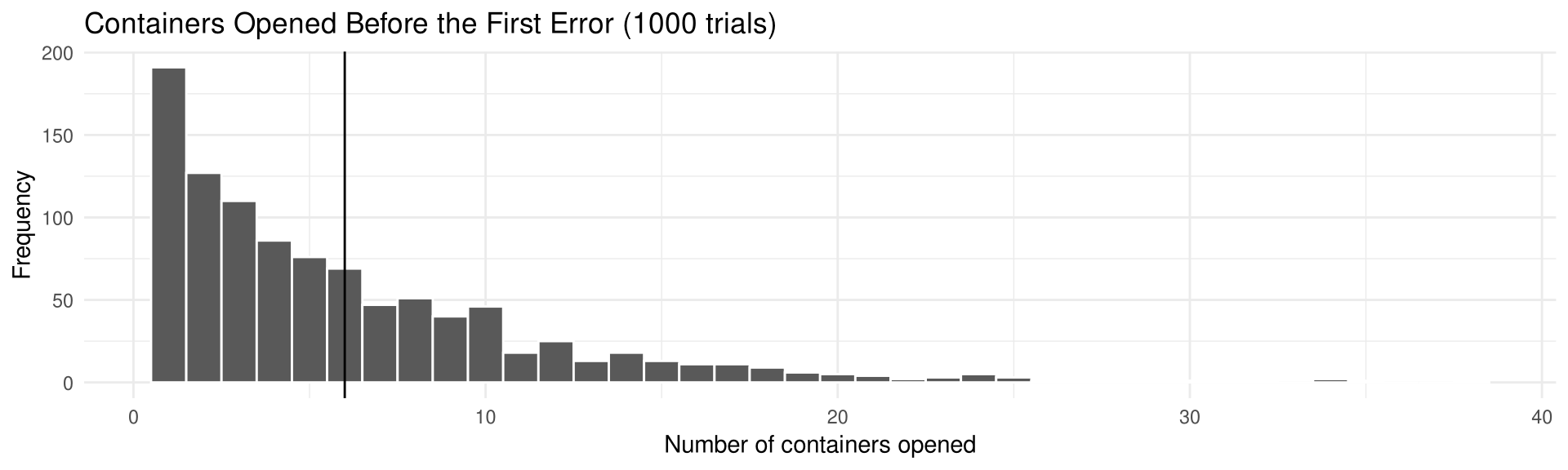
At a container terminal, one container in six has an error in its shipping documents (hypothetical data). An inspector opens containers one at a time until the first documentation error appears. Using simulation, find the average number of containers opened. Try the experiment 20 times.

Example 14-6

Solution

Step 1. List all possible outcomes for one container. Number the six equally likely inspection results 1, 2, 3, 4, 5, 6, and let 6 stand for a documentation error.

Step 2. Determine the probabilities. Each outcome has a probability of \dfrac{1}{6}.

Step 3. Set up a correspondence between the random numbers and the outcomes. Use random numbers 1 through 6; omit the numbers 7, 8, 9 and 0.

Step 4. Select a block of random numbers and count each digit 1 through 6 until the first 6 is obtained. For example, the block 40719236 means that 5 containers were opened, since 0, 7 and 9 are omitted and the inspections are 4, 1, 2, 3, 6.

Example 14-6

Solution

Step 4 (continued). The 20 trials produced by the simulation below are:

Trial  Containers opened    Trial  Containers opened
  1            1             11            5
  2            7             12           11
  3            4             13            8
  4            9             14            8
  5            2             15            1
  6            2             16            6
  7            1             17            5
  8            2             18           12
  9           11             19            8
 10            9             20            2
                                  Total  114

Example 14-6

Solution

Step 5. Compute the results and draw a conclusion. Here you must find the average:

\bar{X} = \frac{\Sigma X}{n} = \frac{114}{20} = 5.7

Hence, the average is about 6 containers.

Note: the waiting time to the first success has expected value \dfrac{1}{p} = \dfrac{1}{1/6} = 6, so the theoretical average is 6. If this experiment is done many times, say 1000 times, the results should be closer to the theoretical result.

Example 14-6

Solution

Same experiment in R

set.seed(23)
containers_opened <- rgeom(20, prob = 1/6) + 1
containers_opened

 [1]  1  7  4  9  2  2  1  2 11  9  5 11  8  8  1  6  5 12  8  2

sum(containers_opened)

[1] 114

mean(containers_opened)

[1] 5.7

rgeom() counts the failures before the first success, so adding 1 gives the number of containers actually opened. No loop is needed.

Example 14-6

Solution

Prepare data — 1000 trials instead of 20

set.seed(23)
many_inspections <- rgeom(1000, prob = 1/6) + 1
mean(many_inspections)

[1] 6.059

With 1000 trials the average is 6.059, much closer to the theoretical 6 than the 5.7 of 20 trials.

Example 14-6

Solution

Output figure — the vertical line marks the theoretical average of 6

ggplot(data.frame(many_inspections), aes(many_inspections)) +
  geom_histogram(binwidth = 1, color = "white") +
  geom_vline(xintercept = 6) +
  labs(title = "Containers Opened Before the First Error (1000 trials)",
       x = "Number of containers opened", y = "Frequency")

Example 14-7

Finding the Right Pallet

A picker at a distribution centre is told that a customer’s order is on one of four identical pallets. She checks the pallets one at a time, in random order, until she finds the order. Find the average number of pallets checked. Try the experiment 25 times. (hypothetical data)

Example 14-7

Solution

Step 1. List all possible outcomes of the experiment. They are pallet 1, pallet 2, pallet 3 and pallet 4.

Step 2. Determine the probability of each outcome. Since a pallet is checked at random and there are four pallets, the probability of checking each one first is \dfrac{1}{4}.

Step 3. Set up a correspondence between the random numbers and the outcomes. Number the pallets 1 through 4 and assume that the order is on pallet 2. The picker does not know this, so she checks the pallets in random order. For the simulation, read a sequence of random digits using only 1 through 4, skipping any repeat, until the digit 2 is reached.

Example 14-7

Solution

Step 4. Repeat the experiment 24 more times. The 25 trials produced by the simulation below are:

Trial  Pallets checked    Trial  Pallets checked
  1           2            14           4
  2           2            15           3
  3           3            16           3
  4           4            17           3
  5           2            18           3
  6           1            19           4
  7           3            20           4
  8           1            21           3
  9           2            22           2
 10           3            23           3
 11           4            24           2
 12           2            25           3
 13           1                  Total  67

Example 14-7

Solution

Step 5. Compute any statistics and state the conclusions. Find the average:

\bar{X} = \frac{\Sigma X}{n} = \frac{2 + 2 + \cdots + 3}{25} = \frac{67}{25} = 2.68

The theoretical average is 2.5, since the order is equally likely to be found on the first, second, third or fourth pallet checked. Again, only 25 repetitions were used; more repetitions should give a result closer to the theoretical average.

Example 14-7

Solution

Same experiment in R

set.seed(1407)
pallets_checked <- replicate(25, which(sample(4) == 2))

pallets_checked

 [1] 2 2 3 4 2 1 3 1 2 3 4 2 1 4 3 3 3 3 4 4 3 2 3 2 3

sum(pallets_checked)

[1] 67

mean(pallets_checked)

[1] 2.68

mean(1:4)

[1] 2.5

sample(4) shuffles the four pallets into a checking order, and which() reports the position at which the order turns up. The last line is the theoretical average.

Example 14-8

A Scratch-Card Promotion

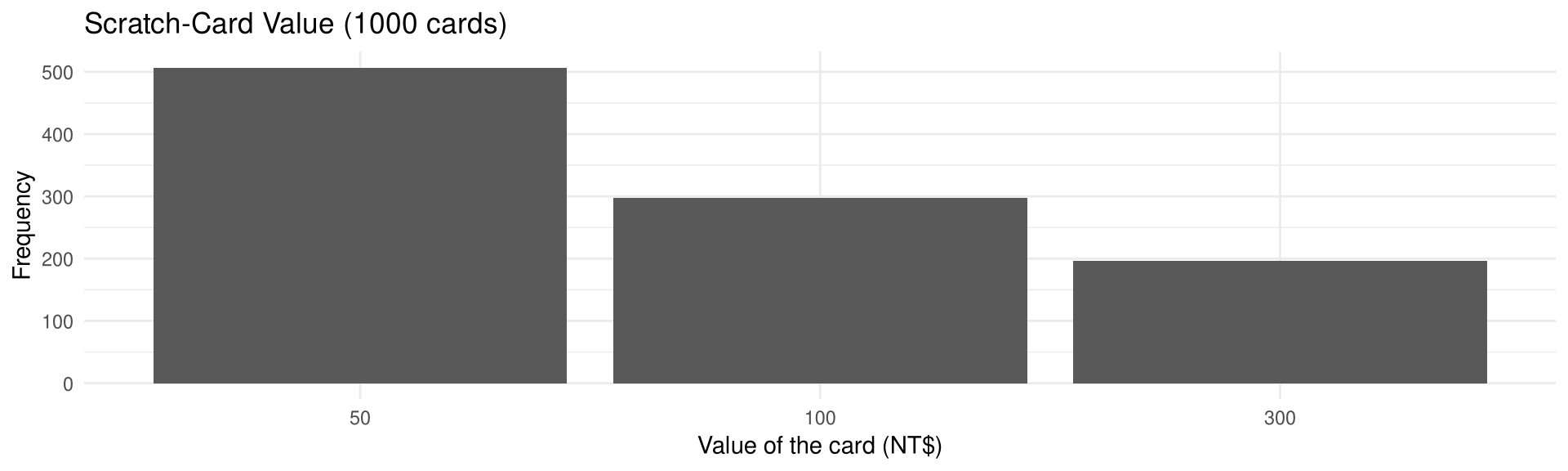
A convenience-store chain runs a scratch-card promotion. Of every 10 cards, five are worth NT$50, three are worth NT$100 and two are worth NT$300 (hypothetical data). A customer scratches one card at random. What is the expected value of a card? Perform the experiment 25 times.

Example 14-8

Solution

Step 1. List all possible outcomes. They are NT$50, NT$100 and NT$300.

Step 2. Assign the probabilities to each outcome:

P(50) = \frac{5}{10} \qquad P(100) = \frac{3}{10} \qquad P(300) = \frac{2}{10}

Step 3. Set up a correspondence between the random numbers and the outcomes. Use random numbers 1 through 5 to represent an NT$50 card, 6 through 8 to represent an NT$100 card, and 9 and 0 to represent an NT$300 card.

Example 14-8

Solution

Step 4. Select 25 random numbers and tally the results.

Number      Results (NT$)
96569       300, 100, 50, 100, 300
56685       50, 100, 100, 100, 50
53749       50, 50, 100, 50, 300
52625       50, 50, 100, 50, 50
43420       50, 50, 50, 50, 300

Step 5. Compute the average:

\bar{X} = \frac{\Sigma X}{n} = \frac{300 + 100 + 50 + \cdots + 300}{25} = \frac{2600}{25} = 104

Hence, the simulated average value of a card is NT$104.

Example 14-8

Solution

Recall that using the expected value formula E(X) = \Sigma[X \cdot P(X)] gives a theoretical average of

E(X) = (0.5)(50) + (0.3)(100) + (0.2)(300) = 115

Reproduce the 25 draws in R

set.seed(108)
card_digits <- sample(0:9, size = 25, replace = TRUE)
card_value  <- ifelse(card_digits %in% 1:5, 50,
                      ifelse(card_digits %in% 6:8, 100, 300))

card_value

 [1] 300 100  50 100 300  50 100 100 100  50  50  50 100  50 300  50  50 100  50
[20]  50  50  50  50  50 300

sum(card_value)

[1] 2600

mean(card_value)

[1] 104

ifelse() applies the correspondence of Step 3: digits 1 to 5 give NT$50, 6 to 8 give NT$100, and 9 and 0 give NT$300.

Example 14-8

Solution

Prepare data — 1000 cards instead of 25

set.seed(1418)
many_cards <- sample(c(50, 100, 300), size = 1000, replace = TRUE,
                     prob = c(0.5, 0.3, 0.2))
mean(many_cards)

[1] 113.85

Over 1000 cards the average is 113.85, close to the theoretical NT$115.

Example 14-8

Solution

Output figure

ggplot(data.frame(many_cards), aes(factor(many_cards))) +
  geom_bar() +
  labs(title = "Scratch-Card Value (1000 cards)",
       x = "Value of the card (NT$)", y = "Frequency")

Simulation Is an Approximation

Caution

Remember that simulation techniques do not give exact results. The more times the experiment is performed, the closer the actual results should be to the theoretical results. (Recall the law of large numbers.)

Example	Simulated result	Theoretical result
14-6 Inspecting containers	5.7 containers	6 containers
14-7 Finding a pallet	2.68 pallets	2.5 pallets
14-8 Scratch card	NT$104	NT$115

The Monty Hall Problem in R

On a game show the host gives a contestant a choice of three doors. A prize is behind one door. After the contestant selects a door, the host opens one of the other doors with no prize behind it and asks whether the contestant wants to switch. By switching, the probability of winning is \dfrac{2}{3} and the probability of losing is \dfrac{1}{3}.

set.seed(2023)
prize_door <- sample(1:3, size = 10000, replace = TRUE)
first_pick <- sample(1:3, size = 10000, replace = TRUE)

mean(first_pick != prize_door)

[1] 0.6672

Switching wins exactly when the first pick was wrong, so the door the host opens never has to be simulated. The simulated win rate is 0.6672, against the theoretical \dfrac{2}{3} \approx 0.667.

Section 14-4: Big Data

What Is Big Data?

With the advent of computers and their expanding capacity, companies can secure large amounts of data every day. Hence a relatively new field of applications of data, called big data, is emerging.

Big Data

Any kind of data which has these three characteristics is defined as big data:

1. There is an extremely large volume of data.
2. There is an extremely high velocity of data. (This means that the size of the data set is increasing very rapidly.)
3. There is an extremely wide variety of data in the data set.

The 3 V’s, and a Fourth

Volume, Velocity, Variety and Variability

V	Meaning
Volume	The data set is extremely large
Velocity	The size of the data set is increasing very rapidly
Variety	The data set contains an extremely wide variety of data
Variability	The data can be collected at various times, such as monthly, seasonally, or per event

The first three characteristics are known as the 3 V’s of big data, first developed by industrial analyst Doug Laney.

Structured and Unstructured Data

Two Kinds of Data

Structured data are data that can be displayed in the form of tables using rows and columns. Numbers, names, dates, genders, income and groups of words are examples.

Unstructured data are data in which words and images are used. Text messages, comments about a business, emails, photographs, and data that include various profiles of situations where words and images are used are some examples.

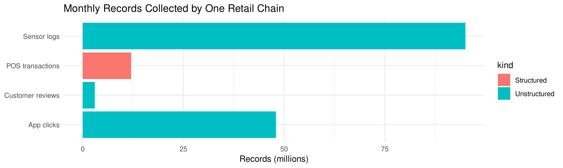
Most of what an organization collects today is unstructured: for every transaction record that fits neatly into rows and columns there are many more reviews, emails, photographs, voice recordings and sensor logs that do not.

Structured and Unstructured Data in R

structured_orders <- data.frame(
  order_id = 1:3,
  date     = c("2026-03-05", "2026-03-06", "2026-03-06"),
  amount   = c(245, 138, 1020),
  store    = c("Taipei", "Kaohsiung", "Taipei")
)
structured_orders

  order_id       date amount     store
1        1 2026-03-05    245    Taipei
2        2 2026-03-06    138 Kaohsiung
3        3 2026-03-06   1020    Taipei

unstructured_reviews <- c("the delivery was late but the staff were kind",
                          "great coffee, terrible parking")
nchar(unstructured_reviews)

[1] 45 30

The orders sort, average and join at once; the reviews do not.

Structured and Unstructured Data in R

Output figure — one retail chain’s monthly data volume (hypothetical data)

monthly_records <- data.frame(
  source   = c("POS transactions", "App clicks", "Customer reviews", "Sensor logs"),
  kind     = c("Structured", "Unstructured", "Unstructured", "Unstructured"),
  millions = c(12, 48, 3, 95)
)

ggplot(monthly_records, aes(millions, source, fill = kind)) +
  geom_col() +
  labs(title = "Monthly Records Collected by One Retail Chain",
       x = "Records (millions)", y = NULL)

Where Big Data Comes From

Big data sets are obtained from a variety of sources.

• Web-connected devices. Every time you conduct a web search, the sites you visit are recorded.
• Marketing and sales systems, which log every transaction, every click and every returned item.
• Government open-data portals, which publish large administrative data sets for anyone to download.

Three Aspects of Big Data

What Must Be Considered

1. How the data can be collected.
2. How the data can be stored so that they can be retrieved.
3. How the data can be analyzed or used easily.

Aspect 1: Collecting the Data

Data can be collected on a day-to-day basis. In manufacturing processes, the information about the use of a credit card is recorded. In health care, records of illnesses, treatments and successes of patient treatments are recorded.

Machine-Generated and Human-Generated Data

Data can be machine-generated, computer-generated or human-generated; sometimes data are obtained by a combination of human- and machine-generated processes.

• Machine-generated data can be obtained at the point of sale of items.
• Human-generated data can be obtained when a human collects the data and inputs it into a computer for storage.

Aspect 2: Storing the Data

The second aspect of big data is how and where it is stored. It is necessary to structure the data so that they can be retrieved to be analyzed. This is a complicated process, since a large variety of data is collected.

For example, a single credit card transaction could include the customer’s name, address, phone number, type of card used, credit card number, the items purchased, the amount of the purchase, and the time and date of purchase.

• Storage is increasingly rented from cloud providers rather than built in-house, because the volume grows faster than any one organization’s own servers.
• Retrieving the right slice of a very large set means spreading it over many machines and processing the pieces in parallel, which is what distributed computing frameworks are designed to do.

Aspect 3: Analyzing the Data

Big data sets are analyzed to give information that helps business owners make better decisions and run their businesses more efficiently.

An Illustration: Routing a Delivery Fleet

Consider a parcel carrier whose vans carry sensors that record every stop, every idling minute and every door opening. One van’s log for one day is of little interest on its own. Pooled over thousands of vans and millions of stops, the same records show which turns, which delivery windows and which street sequences cost the most time and fuel.

The output of the analysis is a route plan: the order in which each driver should make the day’s stops. Shorter routes mean less fuel, fewer driving hours and less wear on the vehicles — a saving that is invisible in any single day’s data but substantial across a fleet over a year.

Where Big Data Is Used

Applications

Field	Use of big data analysis
Banking	Boost customer satisfaction with the banks’ services, minimize fraud, keep up with the services of other banks
Education	Identify potential dropouts before they leave and provide services to keep them in school; track student progress against other schools; find better methods of student evaluation
Government	Manage utilities and agencies, reduce traffic congestion, reduce crime
Health care	Improve patient care by keeping records of illnesses, prescriptions, treatments and recoveries; give doctors quick, accurate access to patient health records
Manufacturing	Boost output, minimize waste, make sound decisions about products and services
Retail sales	Find the most effective way to handle customer complaints and bring back customers who no longer use the business

Big Data Is Here to Stay

Many of the statistical techniques in this book, along with other techniques such as optimization, affinity analysis and forecasting, can be used with big data to make our lives easier and more exciting.

Important Terms

Chapter 14 Vocabulary

biased sample · big data · cluster sample · convenience sample · double sampling · Monte Carlo method · multistage sampling · random sample · sequence sampling · simulation technique · stratified sample · structured data · systematic sample · unbiased sample · unstructured data

Key Takeaways

Key point

• A sample is a subgroup of the population; sampling saves time and money, yields information that could not be obtained otherwise, and allows more detailed study
• For a sample to be random, every member of the population must have an equal chance of being selected; a randomly chosen sample is unbiased, and a sample chosen with systematic error is biased
• Four kinds of bias: sampling or selection, nonresponse, response or interviewer, and volunteer bias
• The four basic sampling methods are random, systematic (every kth element after a random start), stratified (random selection within homogeneous strata) and cluster (a preexisting natural group)
• Other methods are sequence sampling (quality control), double sampling (screen, then sample), multistage sampling (a combination of methods) and convenience sampling

Key Takeaways

Key point

• Survey questions must avoid bias, confusing words, double-barreled questions, double negatives and improper ordering; timing, known identity, and open- versus closed-ended wording also change the answers
• A simulation technique uses a probability experiment to mimic a real-life situation; the Monte Carlo method is a simulation technique using random numbers, carried out in five steps
• Simulation gives approximate results: 5.7 containers against a theoretical 6 in Example 14-6, 2.68 pallets against 2.5 in Example 14-7, and NT$104 against NT$115 in Example 14-8; the law of large numbers closes the gap as repetitions increase
• Big data is defined by the 3 V’s — volume, velocity and variety — with variability often added; data are structured when they fit into rows and columns and unstructured when they are text, images or other free-form records
• Big data must be collected, stored and analyzed, and is used in banking, education, government, health care, manufacturing and retail

Acknowledgement

• Copyright notice. These teaching materials follow the organization and terminology of Bluman, A. G. (2023). Elementary statistics: A step by step approach (11th ed.). McGraw Hill. All rights in the original work are reserved by its authors and publishers.

• Original examples. Every worked example, data set, and R script in these slides was written for this course. The data are hypothetical unless stated otherwise.

• Non-commercial use only. These materials are strictly intended for educational purposes and must not be used for commercial gain or profit.

• Proper attribution. Any reproduction, distribution, or use of these materials must provide proper attribution to the original source.