Statistics

Chapter 3: Data Description

Yu-You Liou

Shih Chien University

2026-10-08

Overview

Chapter 3 shows the statistical methods used to summarize data — measures of average, measures of variation, and measures of position.

Section	Topics
3-1	Mean, median, mode, midrange, weighted mean; distribution shapes
3-2	Range, variance, standard deviation, coefficient of variation; range rule of thumb; Chebyshev’s theorem; empirical rule; linear transformations
3-3	Standard scores, percentiles, deciles, quartiles, outliers
3-4	Five-number summary and boxplots

Chapter Objectives

After completing this chapter, you should be able to

1. Summarize data, using measures of central tendency, such as the mean, median, mode, and midrange.
2. Describe data, using measures of variation, such as the range, variance, and standard deviation.
3. Identify the position of a data value in a data set, using various measures of position, such as percentiles, deciles, and quartiles.
4. Use the techniques of exploratory data analysis, including boxplots and five-number summaries, to discover various aspects of data.

Section 3-1: Measures of Central Tendency

Statistics and Parameters

Loosely stated, the average means the center of the distribution or the most typical case. Measures of average are also called measures of central tendency and include the mean, median, mode, and midrange.

Statistic and Parameter

• A statistic is a characteristic or measure obtained by using the data values from a sample.
• A parameter is a characteristic or measure obtained by using all the data values from a specific population.

General Rounding Rule

Rounding should not be done until the final answer is calculated. Rounding in intermediate steps tends to increase the difference between that answer and the exact one.

The Mean

The mean, also known as the arithmetic average, is found by adding the values of the data and dividing by the total number of values.

The Mean

The mean is the sum of the values, divided by the total number of values.

The sample mean, denoted by \bar{X}, is a statistic: \bar{X} = \frac{X_1 + X_2 + \cdots + X_n}{n} = \frac{\Sigma X}{n}

The population mean, denoted by \mu, is a parameter: \mu = \frac{X_1 + X_2 + \cdots + X_N}{N} = \frac{\Sigma X}{N}

Rounding Rule for the Mean

Rounding Rule for the Mean

The mean should be rounded to one more decimal place than occurs in the raw data. If the raw data are whole numbers, round the mean to the nearest tenth; if the data are in tenths, round to the nearest hundredth.

Greek letters denote parameters; Roman letters denote statistics. Assume the data are obtained from samples unless otherwise specified.

Example 3-1

Monthly Revenue of a Coffee Chain

The figures show last month’s revenue (in NT$ million) for the nine branches of a coffee chain. Find the mean.

2.8   3.5   4.1   2.6   5.0   3.9   4.4   3.2   4.7

(hypothetical data)

Example 3-1

Solution

Solve

coffee_revenue <- c(2.8, 3.5, 4.1, 2.6, 5.0, 3.9, 4.4, 3.2, 4.7)

sum(coffee_revenue)

[1] 34.2

mean(coffee_revenue)

[1] 3.8

\bar{X} = \frac{\Sigma X}{n} = \frac{34.2}{9} = 3.8

The mean monthly revenue for the nine branches is NT$3.8 million.

Example 3-2

Export Value of a Trading Company

The data show the annual export value (in NT$ million) of a small trading company over a 5-year period. Find the mean.

486   512   545   578   614

(hypothetical data)

Example 3-2

Solution

Solve

export_value <- c(486, 512, 545, 578, 614)

sum(export_value)

[1] 2735

mean(export_value)

[1] 547

\bar{X} = \frac{\Sigma X}{n} = \frac{2735}{5} = 547

The mean annual export value over the 5-year period is NT$547 million.

The Mean for Grouped Data

The procedure for finding the mean for grouped data assumes that the mean of all the raw data values in each class is equal to the midpoint of the class.

Procedure — Finding the Mean for Grouped Data

1. Make a table with columns A (class), B (frequency f), C (midpoint X_m), D (f \cdot X_m).
2. Find the midpoint of each class and place it in column C.
3. Multiply the frequency by the midpoint for each class; place the product in column D.
4. Find the sum of column D.
5. Divide the sum of column D by the sum of the frequencies.

\bar{X} = \frac{\Sigma f \cdot X_m}{n}

Example 3-3

Revenue of Night Market Stalls

The frequency distribution shows last month’s revenue (in NT$10,000) for 25 stalls in a night market. Find the mean.

Class boundaries    Frequency
    9.5-14.5             8
   14.5-19.5             7
   19.5-24.5             5
   24.5-29.5             3
   29.5-34.5             2
             Total      25

(hypothetical data)

Back to Example 3-9

Example 3-3

Solution

Prepare data

f  <- c(8, 7, 5, 3, 2)
Xm <- c(12, 17, 22, 27, 32)

f * Xm

[1]  96 119 110  81  64

Example 3-3

Solution

Solve

sum(f)

[1] 25

sum(f * Xm)

[1] 470

sum(f * Xm) / sum(f)

[1] 18.8

\bar{X} = \frac{\Sigma f \cdot X_m}{n} = \frac{470}{25} = 18.8

The mean monthly revenue is NT$188,000 per stall.

The Median

An article reported that the median income for college professors was $82,974: one-half of all professors surveyed earned more than that, and one-half earned less.

Data Array and Median

When the data set is ordered from lowest to highest, it is called a data array.

The median is the midpoint of the data array. The symbol for the median is MD.

Procedure — Finding the Median

1. Arrange the data values in ascending order.
2. Determine the number of values in the data set.
3. If n is odd, select the middle data value as the median. If n is even, find the mean of the two middle values.

Example 3-4

Passengers at MRT Stations

The data show the average number of daily passengers (in thousands) entering seven MRT stations. Find the median.

42   57   38   61   49   55   44

(hypothetical data)

Example 3-4

Solution

Solve

mrt_passengers <- c(42, 57, 38, 61, 49, 55, 44)

sort(mrt_passengers)

[1] 38 42 44 49 55 57 61

length(mrt_passengers)

[1] 7

median(mrt_passengers)

[1] 49

There are an odd number of data values, namely 7, so the middle data value is the median: MD = 49.

The median number of daily passengers is 49 thousand.

Example 3-5

Container Throughput

The number of containers (in thousands of TEU) handled by a port over eight quarters is as follows. Find the median.

146   133   171   119   154   126   162   140

(hypothetical data)

Example 3-5

Solution

Solve

containers_teu <- c(146, 133, 171, 119, 154, 126, 162, 140)

sort(containers_teu)

[1] 119 126 133 140 146 154 162 171

length(containers_teu)

[1] 8

median(containers_teu)

[1] 143

The middle two data values are 140 and 146, so

MD = \frac{140 + 146}{2} = \frac{286}{2} = 143

The median throughput is 143 thousand TEU.

The Mode

The third measure of average is the mode — sometimes said to be the most typical case.

Mode

The value that occurs most often in a data set is called the mode.

• Unimodal — only one value occurs with the greatest frequency.
• Bimodal — two values occur with the same greatest frequency; both are modes.
• Multimodal — more than two values occur with the same greatest frequency.
• No mode — no data value occurs more than once.

Caution

When no value occurs more than once, do not say that the mode is zero. That would be incorrect, because in some data, such as temperature, zero can be an actual value.

Example 3-6

Food Delivery Times

The delivery times, in minutes, for seven randomly selected food delivery orders are shown. Find the mode.

32   28   35   28   41   37   26

(hypothetical data)

Example 3-6

Solution

Solve

delivery_time <- c(32, 28, 35, 28, 41, 37, 26)

sort(delivery_time)

[1] 26 28 28 32 35 37 41

table(delivery_time)

delivery_time
26 28 32 35 37 41 
 1  2  1  1  1  1 

The mode is 28 minutes, because it occurs twice, which is more than any other value.

Example 3-7

Pickers on Duty

The data show the number of pickers on duty at a distribution center over a 15-day period. Find the mode.

18   18   18   18   18
21   23   23   23   24
23   25   26   25   23

(hypothetical data)

Example 3-7

Solution

Solve

pickers <- c(18, 18, 18, 18, 18,
             21, 23, 23, 23, 24,
             23, 25, 26, 25, 23)

table(pickers)

pickers
18 21 23 24 25 26 
 5  1  5  1  2  1 

Since the values 18 and 23 both occur 5 times, the modes are 18 and 23. The data set is said to be bimodal.

Example 3-8

Hotel Ratings

The data show the average customer rating of 8 business hotels on a booking platform. Find the mode.

4.3   3.8   4.6   3.5   4.1   3.9   4.8   4.2

(hypothetical data)

Example 3-8

Solution

Solve

hotel_rating <- c(4.3, 3.8, 4.6, 3.5, 4.1, 3.9, 4.8, 4.2)

table(hotel_rating)

hotel_rating
3.5 3.8 3.9 4.1 4.2 4.3 4.6 4.8 
  1   1   1   1   1   1   1   1 

max(table(hotel_rating))

[1] 1

Since each value occurs only once, there is no mode.

The Modal Class

Modal Class

The mode for grouped data is the modal class — the class with the largest frequency.

Example 3-9

Revenue of Night Market Stalls

Find the modal class for the frequency distribution of night market stall revenue shown in Example 3-3.

Example 3-9

Solution

Solve

f

[1] 8 7 5 3 2

max(f)

[1] 8

Since the class 9.5–14.5 has the largest frequency, 8, it is the modal class. Sometimes the midpoint of the class is used; in this case it is 12.

The Mode for Nominal Data

The mode is the only measure of central tendency that can be used in finding the most typical case when the data are nominal or categorical.

Example 3-10

Payment Methods

The data show the payment method chosen by the customers of an online store on a single day. Find the mode.

Method            Number
Credit card         214
Mobile payment      168
Cash                 95
Store credit         32
Bank transfer        11

(hypothetical data)

Example 3-10

Solution

Solve

data.frame(method = c("Credit card", "Mobile payment", "Cash",
                      "Store credit", "Bank transfer"),
           number = c(214, 168, 95, 32, 11))

          method number
1    Credit card    214
2 Mobile payment    168
3           Cash     95
4   Store credit     32
5  Bank transfer     11

Since the credit card category has the largest frequency, 214, the most typical payment method was the credit card.

Outliers and the Mean

An extremely high or extremely low data value in a data set can have a striking effect on the mean. These extreme values are called outliers. A method for identifying outliers is given in Section 3-3.

Example 3-11

Salaries at a Trading Firm

A small trading firm consists of the owner, the manager, a sales representative, and two clerks, whose monthly salaries in NT dollars are listed here. (Assume that this is the entire population.) Find the mean, median, and mode.

Position            Salary
Owner              180,000
Manager             72,000
Sales rep           48,000
Clerk               35,000
Clerk               35,000

(hypothetical data)

Example 3-11

Solution

Solve

salary <- c(180000, 72000, 48000, 35000, 35000)

mean(salary)

[1] 74000

median(salary)

[1] 48000

table(salary)

salary
 35000  48000  72000 180000 
     2      1      1      1 

\mu = \frac{\Sigma X}{N} = \frac{370{,}000}{5} = 74{,}000

The mean is NT$74,000, the median is NT$48,000, and the mode is NT$35,000.

Example 3-11

Solution

Interpretation

The mean is much higher than the median or the mode, because the extremely high salary of the owner tends to raise the value of the mean. In this and similar situations, the median should be used as the measure of central tendency.

The Midrange

Midrange

The midrange is defined as the sum of the lowest and highest values in the data set, divided by 2. The symbol MR is used for the midrange.

MR = \frac{\text{lowest value} + \text{highest value}}{2}

The midrange is a very rough estimate of the average and can be affected by one extremely high or low value.

Example 3-12

Flight Cancellations

The number of flight cancellations recorded by an airline in each of five months is shown. Find the midrange.

6   41   97   112   58

(hypothetical data)

Example 3-12

Solution

Solve

cancellations <- c(6, 41, 97, 112, 58)

min(cancellations)

[1] 6

max(cancellations)

[1] 112

(min(cancellations) + max(cancellations)) / 2

[1] 59

MR = \frac{6 + 112}{2} = \frac{118}{2} = 59

The midrange for the number of flight cancellations is 59.

Example 3-13

Containers Loaded

The number of containers (in thousands) loaded at an export terminal in each of five years is shown. Find the midrange.

318   742   906   455   264

(hypothetical data)

Example 3-13

Solution

Solve

containers_loaded <- c(318, 742, 906, 455, 264)

min(containers_loaded)

[1] 264

max(containers_loaded)

[1] 906

(min(containers_loaded) + max(containers_loaded)) / 2

[1] 585

MR = \frac{264 + 906}{2} = \frac{1170}{2} = 585

The midrange is 585 thousand containers.

The Weighted Mean

Sometimes you must find the mean of a data set in which not all values are equally represented.

Weighted Mean

Find the weighted mean of a variable X by multiplying each value by its corresponding weight and dividing the sum of the products by the sum of the weights.

\bar{X} = \frac{w_1 X_1 + w_2 X_2 + \cdots + w_n X_n}{w_1 + w_2 + \cdots + w_n} = \frac{\Sigma wX}{\Sigma w}

where w_1, w_2, \ldots, w_n are the weights and X_1, X_2, \ldots, X_n are the values.

Example 3-14

Grade Point Average

An ETP student received an A in International Trade Practice (4 credits), a B in Business Statistics (3 credits), a C in Managerial Accounting (3 credits), and a B in Business English Presentation (2 credits). Assuming A = 4 grade points, B = 3, C = 2, D = 1, and F = 0, find the student’s grade point average.

Example 3-14

Solution

Solve

credits      <- c(4, 3, 3, 2)
grade_points <- c(4, 3, 2, 3)

sum(credits * grade_points) / sum(credits)

[1] 3.083333

\bar{X} = \frac{\Sigma wX}{\Sigma w} = \frac{4 \cdot 4 + 3 \cdot 3 + 3 \cdot 2 + 2 \cdot 3}{4+3+3+2} = \frac{37}{12} \approx 3.1

The grade point average is 3.1.

Table 3-1: Summary of Measures of Central Tendency

Measure	Definition	Symbol(s)
Mean	Sum of values, divided by total number of values	\mu, \bar{X}
Median	Middle point in data set that has been ordered	MD
Mode	Most frequent data value	None
Midrange	Lowest value plus highest value, divided by 2	MR

Properties and Uses of the Mean and Median

The Mean

1. The mean is found by using all the values of the data.
2. The mean varies less than the median or mode when samples are taken from the same population.
3. The mean is used in computing other statistics, such as the variance.
4. The mean for the data set is unique and not necessarily one of the data values.
5. The mean cannot be computed for a frequency distribution that has an open-ended class.
6. The mean is affected by outliers and may not be the appropriate average in these situations.

Properties and Uses of the Mean and Median

The Median

1. The median is used to find the center or middle value of a data set.
2. The median is used when it is necessary to find out whether the data values fall into the upper half or lower half of the distribution.
3. The median is used for an open-ended distribution.
4. The median is affected less than the mean by extremely high or extremely low values.

Properties and Uses of the Mode and Midrange

The Mode

1. The mode is used when the most typical case is desired.
2. The mode is the easiest average to compute.
3. The mode can be used when the data are nominal or categorical, such as religious preference, gender, or political affiliation.
4. The mode is not always unique. A data set can have more than one mode, or the mode may not exist.

The Midrange

1. The midrange is easy to compute.
2. The midrange gives the midpoint.
3. The midrange is affected by extremely high or low values in a data set.

Distribution Shapes

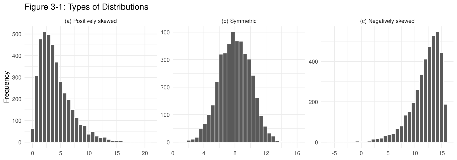
Frequency distributions can assume many shapes. The three most important shapes are positively skewed, symmetric, and negatively skewed (Figure 3-1).

Three Distribution Shapes

• Positively skewed (right-skewed) — the majority of the data values fall to the left of the mean and cluster at the lower end; the tail is to the right. The mean is to the right of the median, and the mode is to the left of the median.
• Symmetric — the data values are evenly distributed on both sides of the mean. When the distribution is unimodal, the mean, median, and mode are the same and lie at the center.
• Negatively skewed (left-skewed) — the majority of the data values fall to the right of the mean and cluster at the upper end; the tail is to the left. The mean is to the left of the median, and the mode is to the right of the median.

Skewness and the Choice of Average

Incomes in the United States are positively skewed: most incomes cluster at the low end, and the few high incomes form a tail on the right. If most students score very high on an examination, the distribution of scores is negatively skewed.

Caution

When a distribution is extremely skewed, the value of the mean is pulled toward the tail, so the median rather than the mean is the more appropriate measure of central tendency. An extremely skewed distribution can also affect other statistics.

Distribution Shapes in R

Prepare data

set.seed(2026)
shapes <- data.frame(
  shape = rep(c("(a) Positively skewed", "(b) Symmetric", "(c) Negatively skewed"),
              each = 4000),
  value = c(rgamma(4000, 2, 0.5), rnorm(4000, 8, 2), 16 - rgamma(4000, 2, 0.5))
)

Distribution Shapes in R

Output figure

ggplot(shapes, aes(value)) +
  geom_histogram(bins = 30, color = "white") +
  facet_wrap(~ shape, scales = "free") +
  labs(title = "Figure 3-1: Types of Distributions", x = NULL, y = "Frequency")

In the skewed panels the mean is pulled toward the long tail, while the median stays near the bulk of the data.

Section 3-2: Measures of Variation

Why Variation Matters

Knowing the average of a data set is not enough to describe it entirely. A shoe store owner who knows that the average size of a man’s shoe is size 10 would not be in business very long if she ordered only size 10 shoes.

In addition to knowing the average, you must know how the data values are dispersed. The measures that determine the spread of the data values are called measures of variation, or measures of dispersion: the range, variance, and standard deviation.

Example 3-15

Comparison of Two Suppliers

A buyer wants to compare two overseas suppliers of packaging film on how long each takes to deliver an order. Six shipments were placed with each supplier. Since only six shipments are involved and no further shipments will be placed under the current contracts, these two groups constitute two small populations. The lead times (in days) are shown. Find the mean of each group.

Supplier A    Supplier B
     9            14
    21            10
     3            13
    15            11
     6            14
    18            10

(hypothetical data)

Back to Example 3-16, Example 3-18, Example 3-19

Example 3-15

Solution

Solve

supplier_a <- c(9, 21, 3, 15, 6, 18)
supplier_b <- c(14, 10, 13, 11, 14, 10)

sum(supplier_a)

[1] 72

mean(supplier_a)

[1] 12

sum(supplier_b)

[1] 72

mean(supplier_b)

[1] 12

\mu_A = \frac{72}{6} = 12 \text{ days} \qquad \mu_B = \frac{72}{6} = 12 \text{ days}

Both means are 12 days.

Example 3-15

Solution

Output figure

lead_times <- data.frame(supplier = rep(c("(a) Supplier A", "(b) Supplier B"), each = 6),
                         days     = c(supplier_a, supplier_b))

ggplot(lead_times, aes(days, supplier)) +
  geom_point() +
  geom_vline(xintercept = 12) +
  labs(title = "Figure 3-2: Examining Data Sets Graphically",
       x = "Lead time (in days)", y = NULL)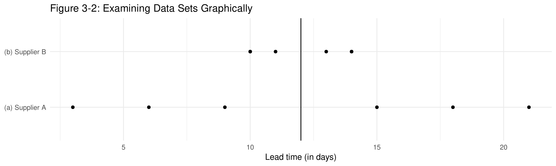

Even though the means are the same, the spread is quite different: supplier B delivers far more consistently.

The Range

Range

The range is the highest value minus the lowest value. The symbol R is used for the range.

R = \text{highest value} - \text{lowest value}

Make sure the range is given as a single number.

Example 3-16

Comparison of Two Suppliers

Find the ranges for the two suppliers in Example 3-15.

Example 3-16

Solution

Solve

max(supplier_a) - min(supplier_a)

[1] 18

max(supplier_b) - min(supplier_b)

[1] 4

For supplier A, R = 21 - 3 = 18 days. For supplier B, R = 14 - 10 = 4 days.

For supplier A, 18 days separate the largest data value from the smallest; for supplier B only 4 days do, which is less than one-fourth of supplier A’s range.

Example 3-17

Parcel Volume

The monthly parcel volumes (in ten thousands) handled by a logistics hub for six selected months are shown. Find the range.

37   62   19   48   55   41

(hypothetical data)

Example 3-17

Solution

Solve

parcels <- c(37, 62, 19, 48, 55, 41)

max(parcels) - min(parcels)

[1] 43

R = 62 - 19 = 43 \text{ (ten thousand parcels)}

One extremely high or one extremely low data value can affect the range markedly, so statisticians use the variance and standard deviation for a more meaningful measure of variability.

Population Variance and Standard Deviation

Data variation is based on the difference or distance each data value is from the mean; this distance is called a deviation, X - \mu. The sum of the deviations about the mean is always zero, so the deviations are squared.

Population Variance and Standard Deviation

The population variance is the average of the squares of the distance each value is from the mean:

\sigma^2 = \frac{\Sigma(X - \mu)^2}{N}

The population standard deviation is the square root of the variance:

\sigma = \sqrt{\sigma^2} = \sqrt{\frac{\Sigma(X - \mu)^2}{N}}

where X = individual value, \mu = population mean, N = population size.

Procedure and Rounding Rule

Procedure — Population Variance and Standard Deviation

1. Find the mean for the data, \mu = \dfrac{\Sigma X}{N}.
2. Find the deviation for each data value, X - \mu.
3. Square each of the deviations, (X - \mu)^2.
4. Find the sum of the squares, \Sigma(X - \mu)^2.
5. Divide by N to get the variance.
6. Take the square root of the variance to get the standard deviation.

Rounding Rule for the Standard Deviation

The final answer should be rounded to one more decimal place than that of the original data.

Example 3-18

Comparison of Two Suppliers

Find the variance and standard deviation for the lead times of supplier A in Example 3-15. The lead times in days were

9   21   3   15   6   18

Example 3-18

Solution

Prepare data

deviation_a <- supplier_a - mean(supplier_a)

deviation_a

[1] -3  9 -9  3 -6  6

deviation_a^2

[1]  9 81 81  9 36 36

sum(deviation_a^2)

[1] 252

Example 3-18

Solution

Solve

sum(deviation_a^2) / 6

[1] 42

sqrt(sum(deviation_a^2) / 6)

[1] 6.480741

\sigma^2 = \frac{252}{6} = 42 \qquad \sigma = \sqrt{42} \approx 6.5

The variance is 42 and the standard deviation is 6.5 days.

Example 3-19

Comparison of Two Suppliers

Find the variance and standard deviation for the lead times of supplier B in Example 3-15. The lead times in days were

14   10   13   11   14   10

Example 3-19

Solution

Solve

deviation_b <- supplier_b - mean(supplier_b)

deviation_b

[1]  2 -2  1 -1  2 -2

deviation_b^2

[1] 4 4 1 1 4 4

sum(deviation_b^2)

[1] 18

Example 3-19

Solution

Solve

sum(deviation_b^2) / 6

[1] 3

sqrt(sum(deviation_b^2) / 6)

[1] 1.732051

\sigma^2 = \frac{18}{6} = 3 \qquad \sigma \approx 1.7

With equal means, a larger \sigma means more spread: supplier A (6.5) exceeds B (1.7).

Sample Variance and Standard Deviation

Dividing by n usually underestimates the population variance, so the sum of squares is divided by n - 1, giving a slightly larger value and an unbiased estimate of the population variance.

Sample Variance and Standard Deviation

s^2 = \frac{\Sigma(X - \bar{X})^2}{n - 1} \qquad s = \sqrt{s^2} = \sqrt{\frac{\Sigma(X - \bar{X})^2}{n - 1}}

where X = individual value, \bar{X} = sample mean, n = sample size.

Example 3-20

Export Orders

The numbers of export orders received last month by five randomly selected sales offices are shown. Find the variance and standard deviation for the data.

14   50   26   38   32

(hypothetical data)

Back to Example 3-21

Example 3-20

Solution

Solve

export_orders <- c(14, 50, 26, 38, 32)
deviation <- export_orders - mean(export_orders)

deviation

[1] -18  18  -6   6   0

deviation^2

[1] 324 324  36  36   0

Example 3-20

Solution

Solve

sum(deviation^2)

[1] 720

var(export_orders)

[1] 180

sd(export_orders)

[1] 13.41641

s^2 = \frac{720}{5 - 1} = 180 \qquad s = \sqrt{180} \approx 13.4

Shortcut (Computational) Formulas

Shortcut Formulas for s^2 and s

s^2 = \frac{n(\Sigma X^2) - (\Sigma X)^2}{n(n-1)} \qquad s = \sqrt{\frac{n(\Sigma X^2) - (\Sigma X)^2}{n(n-1)}}

These are mathematically equivalent to the previous formulas and do not involve using the mean. Note that \Sigma X^2 is not the same as (\Sigma X)^2: \Sigma X^2 means square the values first, then sum; (\Sigma X)^2 means sum the values first, then square the sum.

Example 3-21

Export Orders

The numbers of export orders received last month by five randomly selected sales offices are shown. Find the variance and standard deviation for the data, using the shortcut formula.

14   50   26   38   32

(hypothetical data)

Back to Example 3-20

Example 3-21

Solution

Solve

sum(export_orders)

[1] 160

sum(export_orders^2)

[1] 5840

(5 * 5840 - 160^2) / (5 * 4)

[1] 180

var(export_orders)

[1] 180

s^2 = \frac{5(5840) - 160^2}{5(4)} = \frac{3600}{20} = 180 \qquad s \approx 13.4

The shortcut formula agrees with var(), and with Example 3-20.

Variance and Standard Deviation for Grouped Data

Shortcut Formula for Grouped Data

s^2 = \frac{n(\Sigma f \cdot X_m^2) - (\Sigma f \cdot X_m)^2}{n(n-1)} \qquad s = \sqrt{\frac{n(\Sigma f \cdot X_m^2) - (\Sigma f \cdot X_m)^2}{n(n-1)}}

where X_m is the midpoint of each class and f is the frequency of each class.

Be sure to use the sum of the frequencies for n — not the number of classes.

Example 3-22

Picking Times at a Distribution Center

Find the sample variance and the sample standard deviation for the frequency distribution shown. The data represent the time, in minutes, needed to pick each of 20 randomly selected orders.

  Class      Frequency   Midpoint
  4.5-9.5         2           7
  9.5-14.5        3          12
 14.5-19.5        5          17
 19.5-24.5        4          22
 24.5-29.5        3          27
 29.5-34.5        2          32
 34.5-39.5        1          37

(hypothetical data)

Example 3-22

Solution

Prepare data

f  <- c(2, 3, 5, 4, 3, 2, 1)
Xm <- c(7, 12, 17, 22, 27, 32, 37)

f * Xm

[1] 14 36 85 88 81 64 37

f * Xm^2

[1]   98  432 1445 1936 2187 2048 1369

Example 3-22

Solution

Solve

sum(f)

[1] 20

sum(f * Xm)

[1] 405

sum(f * Xm^2)

[1] 9515

(20 * 9515 - 405^2) / (20 * 19)

[1] 69.14474

sqrt((20 * 9515 - 405^2) / (20 * 19))

[1] 8.315331

s^2 = \frac{20(9515) - 405^2}{20(19)} = \frac{26{,}275}{380} \approx 69.1 \qquad s \approx 8.3

Table 3-2: Summary of Measures of Variation

Measure	Definition	Symbol(s)
Range	Distance between highest value and lowest value	R
Variance	Average of the squares of the distance that each value is from the mean	\sigma^2, s^2
Standard deviation	Square root of the variance	\sigma, s

Uses of the Variance and Standard Deviation

Four Uses

1. They determine the spread of the data, and are useful in comparing two or more data sets to determine which is more variable.
2. They determine the consistency of a variable. In the manufacture of nuts and bolts, the variation in diameters must be small or the parts will not fit together.
3. They determine the number of data values that fall within a specified interval in a distribution — for example, Chebyshev’s theorem shows that at least 75% of the data values fall within 2 standard deviations of the mean.
4. They are used quite often in inferential statistics.

Coefficient of Variation

When two samples have the same units of measure, their standard deviations can be compared directly. To compare the standard deviations of two different variables, use the coefficient of variation.

Coefficient of Variation

The coefficient of variation, denoted by \text{CVar}, is the standard deviation divided by the mean. The result is expressed as a percentage.

\text{CVar} = \frac{s}{\bar{X}} \cdot 100\% \quad \text{(samples)} \qquad \text{CVar} = \frac{\sigma}{\mu} \cdot 100\% \quad \text{(populations)}

Example 3-23

Store Sales in Two Cities

For the stores of a coffee chain in Taipei, the mean monthly revenue is NT$2.68 million with a standard deviation of NT$523,000. For its stores in Kaohsiung, the mean monthly revenue is NT$1.94 million with a standard deviation of NT$417,000. Compute the coefficient of variation for the two cities. Which data set is more variable?

(hypothetical data)

Example 3-23

Solution

Solve

52.3 / 268 * 100

[1] 19.51493

41.7 / 194 * 100

[1] 21.49485

\text{Taipei: } \text{CVar} = \frac{52.3}{268} \cdot 100\% = 19.5\% \qquad \text{Kaohsiung: } \text{CVar} = \frac{41.7}{194} \cdot 100\% = 21.5\%

The variation of the Kaohsiung stores is only slightly larger than the variation of the Taipei stores. (Both revenue figures are expressed in NT$10,000.)

Example 3-24

Hotel Occupancy and Room Rates

For a sample of international hotels in Taipei, the mean occupancy rate is 72.5% with a variance of 27.04, and the mean average daily room rate is NT$4,850 with a variance of 336,400. Compare the variations of the two data sets.

(hypothetical data)

Example 3-24

Solution

Solve

sqrt(27.04) / 72.5 * 100

[1] 7.172414

sqrt(336400) / 4850 * 100

[1] 11.95876

\text{CVar}_{\text{occupancy}} = \frac{\sqrt{27.04}}{72.5} \cdot 100\% = 7.2\% \qquad \text{CVar}_{\text{rate}} = \frac{\sqrt{336{,}400}}{4850} \cdot 100\% = 12.0\%

The variation in the room rates is larger than the variation in the occupancy rates.

Range Rule of Thumb

The Range Rule of Thumb

A rough estimate of the standard deviation is

s \approx \frac{\text{range}}{4}

The rule can also estimate the extreme data values: the smallest data value is approximately \bar{X} - 2s and the largest is approximately \bar{X} + 2s.

Caution

The range rule of thumb is only an approximation and should be used when the distribution of data values is unimodal and roughly symmetric.

The Range Rule of Thumb in R

containers_per_hour <- c(16, 13, 22, 10, 18, 14, 19, 16)

mean(containers_per_hour)

[1] 16

sd(containers_per_hour)

[1] 3.741657

(max(containers_per_hour) - min(containers_per_hour)) / 4

[1] 3

mean(containers_per_hour) - 2 * sd(containers_per_hour)

[1] 8.516685

mean(containers_per_hour) + 2 * sd(containers_per_hour)

[1] 23.48331

The actual standard deviation is 3.7 and the range is 22 - 10 = 12, so the range rule of thumb gives s \approx 3. The mean is 16, so the estimated smallest and largest values are 8.5 and 23.5 — in the ballpark of the actual 10 and 22.

Chebyshev’s Theorem

Chebyshev’s Theorem

The proportion of values from a data set that will fall within k standard deviations of the mean will be at least 1 - \dfrac{1}{k^2}, where k is a number greater than 1 (k is not necessarily an integer).

• At least three-fourths, or 75%, of all data values fall within 2 standard deviations of the mean.
• At least eight-ninths, or 89%, of all data values fall within 3 standard deviations of the mean.

This theorem can be applied to any distribution, regardless of its shape.

Example 3-25

Rents near Campus

The mean monthly rent for a studio apartment near campus is NT$12,000, and the standard deviation is NT$1,500. Find the rent range for which at least 75% of the studios will be listed.

(hypothetical data)

Example 3-25

Solution

Solve

(1 - 1 / 2^2) * 100

[1] 75

12000 - 2 * 1500

[1] 9000

12000 + 2 * 1500

[1] 15000

12{,}000 + 2(1{,}500) = 15{,}000 \qquad 12{,}000 - 2(1{,}500) = 9{,}000

At least 75% of the studios near campus will be listed between NT$9,000 and NT$15,000.

Example 3-26

Fuel Cost per Delivery

A survey of delivery riders found that the mean fuel cost per order was NT$8.00, with a standard deviation of NT$1.20. Using Chebyshev’s theorem, find the minimum percentage of the orders whose fuel cost falls between NT$5.00 and NT$11.00.

(hypothetical data)

Example 3-26

Solution

Solve

k <- (11.00 - 8.00) / 1.20
k

[1] 2.5

(1 - 1 / k^2) * 100

[1] 84

Step 1. 11.00 - 8.00 = 3.00. Step 2. k = \dfrac{3.00}{1.20} = 2.5.

Step 3. 1 - \dfrac{1}{2.5^2} = 1 - \dfrac{1}{6.25} = 1 - 0.16 = 0.84.

Hence, at least 84% of the orders have a fuel cost between NT$5.00 and NT$11.00.

The Empirical (Normal) Rule

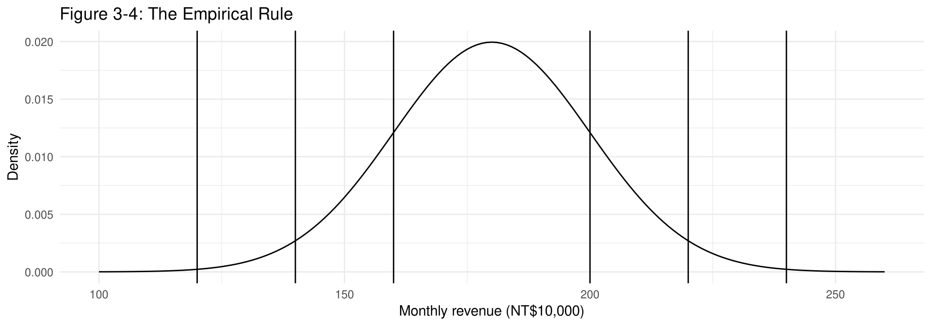
The Empirical Rule

When a distribution is bell-shaped (normal):

• Approximately 68% of the data values will fall within 1 standard deviation of the mean.
• Approximately 95% of the data values will fall within 2 standard deviations of the mean.
• Approximately 99.7% of the data values will fall within 3 standard deviations of the mean.

Because the empirical rule requires the distribution to be approximately bell-shaped, its results are more accurate than those of Chebyshev’s theorem, which applies to all distributions.

The Empirical Rule in R

Prepare data

Suppose the monthly revenue of the stores in a convenience store chain is bell-shaped with a mean of NT$1.8 million and a standard deviation of NT$200,000 (figures below are in NT$10,000).

x <- seq(100, 260, by = 1)
curve <- data.frame(x, density = dnorm(x, 180, 20))

The Empirical Rule in R

Output figure

ggplot(curve, aes(x, density)) +
  geom_line() +
  geom_vline(xintercept = c(120, 140, 160, 200, 220, 240)) +
  labs(title = "Figure 3-4: The Empirical Rule",
       x = "Monthly revenue (NT$10,000)", y = "Density")

Approximately 68% of the stores take between 160 and 200, approximately 95% between 140 and 220, and approximately 99.7% between 120 and 240 (NT$10,000 per month).

Linear Transformation of Data

Sometimes it is necessary to transform data values into other data values — for example, converting Celsius temperatures collected in Canada into Fahrenheit for a study used in the United States. This change is called the linear transformation of the data.

Adding a Constant

When a constant is added to each data value, the mean increases by that constant and the standard deviation does not change.

Multiplying by a Constant

When each data value is multiplied by a constant, the mean of the new data set equals the constant times the old mean, and the standard deviation of the new data set equals the absolute value of the constant times the old standard deviation.

Linear Transformation: Adding a Constant

Suppose a logistics firm employs five part-time packers whose hourly wages are NT$200, NT$185, NT$215, NT$185, and NT$215. After a profitable quarter every packer is given a raise of NT$20 per hour.

hourly_wage <- c(200, 185, 215, 185, 215)
raised_wage <- hourly_wage + 20

mean(hourly_wage)

[1] 200

sd(hourly_wage)

[1] 15

mean(raised_wage)

[1] 220

sd(raised_wage)

[1] 15

The mean rises from NT$200 to NT$220 — exactly the amount added — while the standard deviation stays at 15.

Linear Transformation: Multiplying by a Constant

The same five packers worked 18, 14, 22, 14, and 22 hours last week. Suppose the payroll system records the hours in minutes instead, so every value is multiplied by 60.

weekly_hours   <- c(18, 14, 22, 14, 22)
weekly_minutes <- weekly_hours * 60

mean(weekly_hours)

[1] 18

sd(weekly_hours)

[1] 4

mean(weekly_minutes)

[1] 1080

sd(weekly_minutes)

[1] 240

The mean is multiplied by 60, from 18 hours to 1080 minutes, and the standard deviation is multiplied by 60 as well, from 4 to 240.

Section 3-3: Measures of Position

Locating a Value Within a Distribution

In addition to measures of central tendency and measures of variation, there are measures of position or location. These measures include standard scores, percentiles, deciles, and quartiles. They are used to locate the relative position of a data value in the data set.

If a value is located at the 80th percentile, 80% of the values fall below it and 20% fall above it. The median is the value that corresponds to the 50th percentile.

Standard Scores

A direct comparison of a score of 90 on a music test and 45 on an English exam is impossible, since the exams might not be equivalent in number of questions or value of each question. A comparison of a relative standard can be made using the mean and standard deviation.

z Score (Standard Score)

A z score or standard score for a value is obtained by subtracting the mean from the value and dividing the result by the standard deviation:

z = \frac{\text{value} - \text{mean}}{\text{standard deviation}}

z = \frac{X - \bar{X}}{s} \quad \text{(samples)} \qquad z = \frac{X - \mu}{\sigma} \quad \text{(populations)}

The z score represents the number of standard deviations that a data value falls above or below the mean. If z > 0 the score is above the mean; if z = 0 it equals the mean; if z < 0 it is below the mean.

Example 3-27

Call Handling Times

At a call center’s Taipei site the mean handling time is 4.8 minutes with a standard deviation of 0.6 minute; at its Taichung site the mean is 5.4 minutes with a standard deviation of 0.8 minute. One call in Taipei took 6.3 minutes and one call in Taichung took 6.8 minutes. Compare the relative positions of the two calls.

(hypothetical data)

Example 3-27

Solution

Solve

(6.3 - 4.8) / 0.6

[1] 2.5

(6.8 - 5.4) / 0.8

[1] 1.75

\text{Taipei: } z = \frac{6.3 - 4.8}{0.6} = 2.50 \qquad \text{Taichung: } z = \frac{6.8 - 5.4}{0.8} = 1.75

Since the z score for the Taipei call is higher, that call is relatively longer within its own site than the Taichung call is within its site.

Example 3-28

Daily Revenue of Convenience Stores

For a convenience store chain, the 24-hour branches have a mean daily revenue of NT$52,000 with a standard deviation of NT$5,000, while the campus branches have a mean daily revenue of NT$38,000 with a standard deviation of NT$4,000. Find the relative positions of a 24-hour branch that took NT$45,000 and a campus branch that took NT$33,000.

(hypothetical data)

Example 3-28

Solution

Solve

(45000 - 52000) / 5000

[1] -1.4

(33000 - 38000) / 4000

[1] -1.25

\text{24-hour: } z = \frac{45{,}000 - 52{,}000}{5{,}000} = -1.40 \qquad \text{Campus: } z = \frac{33{,}000 - 38{,}000}{4{,}000} = -1.25

In this case, the campus branch stands relatively higher within its own group than the 24-hour branch does within its group.

When all data for a variable are transformed into z scores, the resulting distribution has a mean of 0 and a standard deviation of 1.

Percentiles

Percentiles

Percentiles divide the data set into 100 equal groups. They are symbolized by P_1, P_2, P_3, \ldots, P_{99}.

Caution

Percentiles are not the same as percentages. If a student gets 72 correct answers out of 100, she obtains a percentage score of 72, which says nothing about her position relative to the class. If a raw score of 72 corresponds to the 64th percentile, then she did better than 64% of the students in her class.

Table 3-3: Percentile Ranks on the Business English Placement Test

Scaled score	Sec. 1: Listening	Sec. 2: Grammar	Sec. 3: Reading	Total scaled	Percentile rank
72	99	98	99	720	99
70	97	95	97	700	96
68	94	91	93	680	92
66	89	85	88	660	87
64	83	78	82	640	80
62	75	70	74	620	72
60	66	60	64	600	63

Percentile ranks published by a business school for the English placement test it gives to incoming students. (hypothetical data)

Table 3-3: Percentile Ranks (continued)

Scaled score	Sec. 1: Listening	Sec. 2: Grammar	Sec. 3: Reading	Total scaled	Percentile rank
58	56	50	54	580	53
56	45	40	43	560	42
54	35	31	33	540	32
52	26	23	25	520	24
50	19	17	18	500	17
48	13	12	13	480	12
46	9	8	9	460	8
44	6	5	6	440	5

Table 3-3: Percentile Ranks (continued)

Scaled score	Sec. 1: Listening	Sec. 2: Grammar	Sec. 3: Reading	Total scaled	Percentile rank
42	4	3	4	420	3
40	2	2	2	400	2
38	1	1	1	380	1
36	1	1	1	360	1
34	1	1	1	340	1
Mean	58.4	59.1	58.7	588
S.D.	6.2	6.8	6.5	62

A student with a scaled score of 64 for section 1 has a percentile rank of 83 — that student did better than 83% of the students who took section 1 of the test.

Example 3-29

Order Values on an E-Commerce Platform

The frequency distribution for the order values (in NT dollars) of 200 randomly selected orders placed on an e-commerce platform is shown here. Construct a percentile graph.

Class boundaries      Frequency
   199.5-399.5            18
   399.5-599.5            52
   599.5-799.5            68
   799.5-999.5            38
   999.5-1199.5           16
  1199.5-1399.5            8
               Total     200

(hypothetical data)

Example 3-29

Solution

Prepare data

\text{Cumulative \%} = \frac{\text{cumulative frequency}}{n} \cdot 100

f <- c(18, 52, 68, 38, 16, 8)

cumsum(f)

[1]  18  70 138 176 192 200

cumsum(f) / 200 * 100

[1]   9  35  69  88  96 100

Example 3-29

Solution

Output figure

percentile_points <- data.frame(boundary    = seq(199.5, 1399.5, by = 200),
                                cum_percent = cumsum(c(0, f)) / 200 * 100)

ggplot(percentile_points, aes(boundary, cum_percent)) +
  geom_line() +
  geom_point() +
  labs(title = "Figure 3-6: Percentile Graph for Example 3-29",
       x = "Class boundaries (NT dollars)", y = "Cumulative percentages")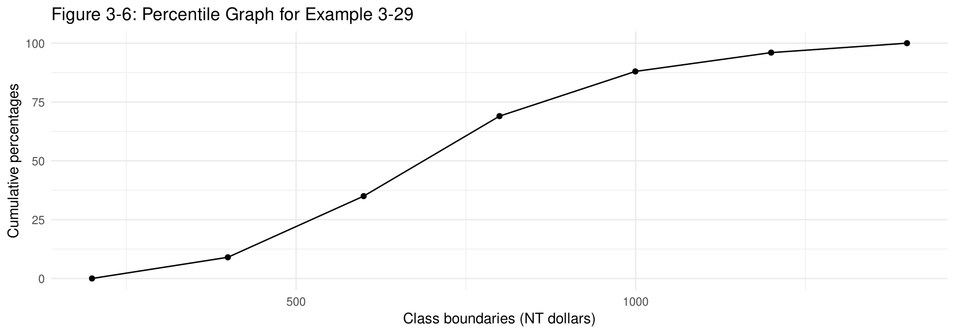

Reading from the graph, an order value of NT$799.50 sits at the 69th percentile, and the 50th percentile falls somewhere between NT$599.50 and NT$799.50.

The Percentile Formula

Percentile Formula

The percentile corresponding to a given value X is computed by using

\text{Percentile} = \frac{(\text{number of values below } X) + 0.5}{\text{total number of values}} \cdot 100

Example 3-30

Product Returns

The number of product returns processed each day by a fulfillment center over a 10-day period is shown. Find the percentile rank of 18.

14   23   9   31   18   27   12   21   35   25

(hypothetical data)

Back to Example 3-31, Example 3-32, Example 3-33

Example 3-30

Solution

Solve

returns <- c(14, 23, 9, 31, 18, 27, 12, 21, 35, 25)

sort(returns)

 [1]  9 12 14 18 21 23 25 27 31 35

sum(returns < 18)

[1] 3

(sum(returns < 18) + 0.5) / 10 * 100

[1] 35

Since there are 3 numbers below the value of 18,

\text{Percentile} = \frac{3 + 0.5}{10} \cdot 100 = 35\text{th percentile}

Hence, the value of 18 is higher than 35% of the data values.

Example 3-31

Product Returns

Using the data in Example 3-30, find the percentile rank of 31.

Example 3-31

Solution

Solve

sum(returns < 31)

[1] 8

(sum(returns < 31) + 0.5) / 10 * 100

[1] 85

There are 8 values below 31; thus

\text{Percentile} = \frac{8 + 0.5}{10} \cdot 100 = 85\text{th percentile}

Therefore, the data value 31 is higher than 85% of the values in the data set.

Finding a Value for a Given Percentile

Procedure — Finding a Data Value Corresponding to a Given Percentile

1. Arrange the data in order from lowest to highest.
2. Substitute into the formula c = \dfrac{n \cdot p}{100}, where n = total number of values and p = percentile.
3. If c is not a whole number, round up to the next whole number and count over to that value from the lowest value. If c is a whole number, use the value halfway between the cth and (c+1)st values.

Example 3-32

Product Returns

Using the data in Example 3-30, find the value corresponding to the 65th percentile.

Example 3-32

Solution

Solve

sort(returns)

 [1]  9 12 14 18 21 23 25 27 31 35

10 * 65 / 100

[1] 6.5

sort(returns)[7]

[1] 25

c = \frac{10 \cdot 65}{100} = 6.5

Since c is not a whole number, round it up to 7. Starting at the lowest value and counting over to the 7th value gives 25. Hence, the value of 25 corresponds to the 65th percentile.

Example 3-33

Product Returns

Using the data in Example 3-30, find the data value corresponding to the 30th percentile.

Example 3-33

Solution

Solve

10 * 30 / 100

[1] 3

(sort(returns)[3] + sort(returns)[4]) / 2

[1] 16

c = \frac{10 \cdot 30}{100} = 3

Since c is a whole number, use the value halfway between the 3rd and 4th values. The halfway value between 14 and 18 is 16, which corresponds to the 30th percentile.

Quartiles and Deciles

Quartiles and Deciles

Quartiles divide the distribution into four equal groups, denoted by Q_1, Q_2, Q_3. Deciles divide the distribution into 10 groups, denoted by D_1, D_2, \ldots, D_9.

• Q_1 = P_{25}, Q_2 = P_{50}, Q_3 = P_{75}
• D_1 = P_{10}, D_2 = P_{20}, …, D_9 = P_{90}
• The median is the same as P_{50} or Q_2 or D_5.

Procedure — Finding Q_1, Q_2, and Q_3

1. Arrange the data in order from lowest to highest.
2. Find the median of the data values. This is Q_2.
3. Find the median of the data values that fall below Q_2. This is Q_1.
4. Find the median of the data values that fall above Q_2. This is Q_3.

Example 3-34

Deliveries per Rider

The numbers of orders delivered in one hour by 9 riders on a food delivery platform are shown. Find Q_1, Q_2, and Q_3.

22   27   19   25   31   24   27   22   26

(hypothetical data)

Back to Example 3-35

Example 3-34

Solution

Solve

deliveries <- c(22, 27, 19, 25, 31, 24, 27, 22, 26)
sorted <- sort(deliveries)

sorted

[1] 19 22 22 24 25 26 27 27 31

median(sorted)

[1] 25

median(sorted[1:4])

[1] 22

median(sorted[6:9])

[1] 27

quantile(deliveries, c(0.25, 0.50, 0.75))

25% 50% 75% 
 22  25  27 

Q_2 = 25 \qquad Q_1 = \frac{22 + 22}{2} = 22 \qquad Q_3 = \frac{27 + 27}{2} = 27

Hence, Q_1 = 22, Q_2 = 25, and Q_3 = 27. The built-in quantile() returns the same three values, so the rest of the chapter simply uses quantile().

The Interquartile Range

Interquartile Range

The interquartile range (IQR) is the difference between the third and first quartiles.

\text{IQR} = Q_3 - Q_1

Quartiles can be used as a rough measure of variability: the IQR is the range of the middle 50% of the data values. Like the standard deviation, the more variable the data set is, the larger the IQR.

Example 3-35

Deliveries per Rider

Find the interquartile range for the data in Example 3-34.

Example 3-35

Solution

Solve

quantile(deliveries, c(0.25, 0.75))

25% 75% 
 22  27 

IQR(deliveries)

[1] 5

\text{IQR} = Q_3 - Q_1 = 27 - 22 = 5

The interquartile range is 5 orders per hour.

Table 3-4: Summary of Position Measures

Measure	Definition	Symbol
Standard score, or z score	Standard deviations a value lies above or below the mean	z
Percentile	Position of a value in hundredths of the distribution	P_n
Decile	Position of a value in tenths of the distribution	D_n
Quartile	Position of a value in fourths of the distribution	Q_n

Outliers

Outlier

An outlier is an extremely high or an extremely low data value when compared with the rest of the data values.

Resistant and Nonresistant Statistics

The mean and standard deviation are affected by outliers, so they are called nonresistant statistics. The median and interquartile range are less affected by outliers, so they are called resistant statistics.

Identifying Outliers

Procedure for Identifying Outliers

1. Arrange the data in order from lowest to highest and find Q_1 and Q_3.
2. Find the interquartile range: \text{IQR} = Q_3 - Q_1.
3. Multiply the IQR by 1.5.
4. Subtract the value obtained in step 3 from Q_1 and add it to Q_3.
5. Check the data set for any value smaller than Q_1 - 1.5(\text{IQR}) or larger than Q_3 + 1.5(\text{IQR}).

Caution

There are no hard-and-fast rules on what to do with outliers, nor complete agreement among statisticians on ways to identify them. When a distribution is normal or bell-shaped, data values beyond 3 standard deviations of the mean can be considered suspected outliers.

Example 3-36

Complaint Tickets

The numbers of complaint tickets received by a customer service team on 8 randomly selected days are shown. Check the set for outliers.

8   4   18   12   57   8   14   18

(hypothetical data)

Example 3-36

Solution

Solve

tickets <- c(8, 4, 18, 12, 57, 8, 14, 18)
Q1 <- quantile(tickets, 0.25)
Q3 <- quantile(tickets, 0.75)

Q1

25% 
  8 

Q3

75% 
 18 

IQR(tickets)

[1] 10

Q1 - 1.5 * IQR(tickets)

25% 
 -7 

Q3 + 1.5 * IQR(tickets)

75% 
 33 

Here Q_1 = 8, Q_3 = 18, \text{IQR} = 10 and 1.5(10) = 15, so the fences are -7 and 33. The data value 57 is greater than 33; hence, it can be considered an outlier.

Section 3-4: Exploratory Data Analysis

Exploratory Data Analysis

The purpose of traditional analysis is to confirm various conjectures about the nature of the data. The purpose of exploratory data analysis is to examine data to find out what information can be discovered about the data, such as the center and the spread.

Exploratory Data Analysis (EDA)

In exploratory data analysis (EDA), data can be organized using a stem and leaf plot. The measure of central tendency used in EDA is the median; the measure of variation is the interquartile range Q_3 - Q_1; and the data are represented graphically using a boxplot (sometimes called a box and whisker plot).

EDA was developed by John Tukey and presented in his book Exploratory Data Analysis (Addison-Wesley, 1977).

The Five-Number Summary and Boxplots

Five-Number Summary

A boxplot involves five specific values, called the five-number summary of the data set:

1. The lowest value of the data set (minimum)
2. Q_1
3. The median
4. Q_3
5. The highest value of the data set (maximum)

Boxplot

A boxplot is a graph of a data set obtained by drawing a horizontal line from the minimum data value to Q_1, drawing a horizontal line from Q_3 to the maximum data value, and drawing a box whose vertical sides pass through Q_1 and Q_3 with a vertical line inside the box passing through the median or Q_2.

Constructing a Boxplot

Procedure — Constructing a Boxplot

1. Find the five-number summary for the data.
2. Draw a horizontal axis and place the scale on the axis. The scale should start on or below the minimum data value and end on or above the maximum data value.
3. Locate the lowest data value, Q_1, the median, Q_3, and the highest data value; draw a box whose vertical sides go through Q_1 and Q_3; draw a vertical line through the median; draw a line from the minimum data value to the left side of the box and from the maximum data value to the right side of the box.

Example 3-37

Revenue of a Beverage Stand

The daily revenue, in NT$1,000, of a beverage stand on 10 randomly selected days is shown. Construct a boxplot for the data.

14   9   26   6   16   12   8   20   16   9

(hypothetical data)

Example 3-37

Solution

Prepare data

daily_revenue <- c(14, 9, 26, 6, 16, 12, 8, 20, 16, 9)

sort(daily_revenue)

 [1]  6  8  9  9 12 14 16 16 20 26

quantile(daily_revenue)

  0%  25%  50%  75% 100% 
   6    9   13   16   26 

The five-number summary is minimum 6, Q_1 = 9, median 13, Q_3 = 16, maximum 26.

Example 3-37

Solution

Output figure

ggplot(data.frame(daily_revenue), aes(daily_revenue)) +
  geom_boxplot() +
  labs(title = "Figure 3-7: Boxplot for Example 3-37",
       x = "Daily revenue (NT$1,000)")

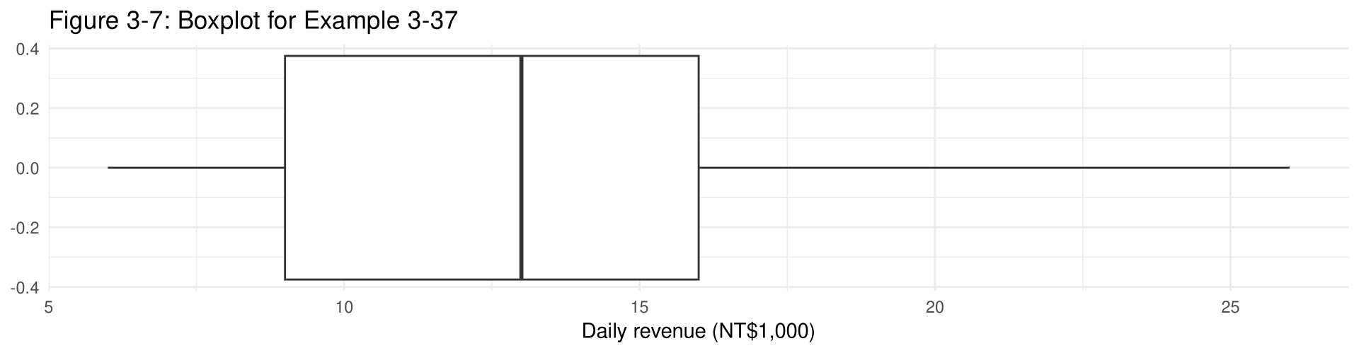
The right whisker is much longer than the left, so the distribution is positively skewed, with a high value of 26 and a low value of 6 thousand NT dollars.

Information Obtained from a Boxplot

Reading a Boxplot

1. The median inside the box
   1. If the median is near the center of the box, the distribution is approximately symmetric.
   2. If the median falls to the left of the center, the distribution is positively skewed.
   3. If the median falls to the right of the center, the distribution is negatively skewed.
2. The lines (whiskers)
   1. If the lines are about the same length, the distribution is approximately symmetric.
   2. If the right line is larger, the distribution is positively skewed.
   3. If the left line is larger, the distribution is negatively skewed.

Example 3-38

Customs Clearance Times at Two Ports

The data shown are the customs clearance times, in hours, for a sample of export shipments at two ports. Compare the distributions by using boxplots.

      Port A                    Port B
 22   26   20   18       32   56   24   16
 24   28   20   26       48   64   56   24

(hypothetical data)

Example 3-38

Solution

Prepare data

port_a <- c(22, 26, 20, 18, 24, 28, 20, 26)
port_b <- c(32, 56, 24, 16, 48, 64, 56, 24)

quantile(port_a, c(0.25, 0.50, 0.75))

25% 50% 75% 
 20  23  26 

quantile(port_b, c(0.25, 0.50, 0.75))

25% 50% 75% 
 24  40  56 

For port A, Q_1 = 20, MD = 23, Q_3 = 26; for port B, Q_1 = 24, MD = 40, Q_3 = 56.

Example 3-38

Solution

Output figure

clearance <- data.frame(port  = rep(c("Port A", "Port B"), each = 8),
                        hours = c(port_a, port_b))

ggplot(clearance, aes(hours, port)) +
  geom_boxplot() +
  labs(title = "Figure 3-8: Boxplots for Example 3-38",
       x = "Customs clearance time (hours)", y = NULL)

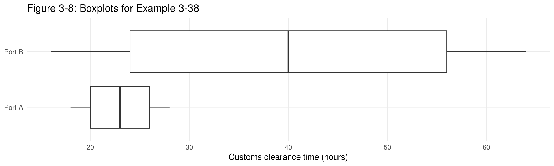
The median clearance time at port B is much higher, and both the interquartile range and the range at port B are much larger than those at port A.

Hinges versus Quartiles

Caution

In exploratory data analysis, hinges are used instead of quartiles to construct boxplots. When the data set consists of an even number of values, hinges are the same as quartiles; hinges for a data set with an odd number of values differ somewhat from quartiles. Since most calculators and computer programs use quartiles, quartiles are used in this textbook.

A modified boxplot can be drawn to check for outliers: the whiskers extend only to the highest and lowest values within 1.5(\text{IQR}) of the box.

Table 3-5: Traditional versus EDA Techniques

Traditional	Exploratory data analysis
Frequency distribution	Stem and leaf plot
Histogram	Boxplot
Mean	Median
Standard deviation	Interquartile range

Important Terms

Chapter 3 Vocabulary

bimodal · boxplot · Chebyshev’s theorem · coefficient of variation · data array · decile · empirical rule · exploratory data analysis (EDA) · five-number summary · interquartile range (IQR) · mean · median · midrange · modal class · mode · multimodal · negatively skewed or left-skewed distribution · nonresistant statistic · outlier · parameter · percentile · population mean · population standard deviation · population variance · positively skewed or right-skewed distribution · quartile · range · range rule of thumb · resistant statistic · sample mean · standard deviation · statistic · symmetric distribution · unimodal · variance · weighted mean · z score or standard score

Key Formulas

Central Tendency

\bar{X} = \frac{\Sigma X}{n} \qquad \mu = \frac{\Sigma X}{N} \qquad \bar{X} = \frac{\Sigma f \cdot X_m}{n}

\bar{X} = \frac{\Sigma wX}{\Sigma w} \qquad MR = \frac{\text{lowest value} + \text{highest value}}{2}

Variation

R = \text{highest value} - \text{lowest value} \qquad \sigma^2 = \frac{\Sigma(X-\mu)^2}{N} \qquad \sigma = \sqrt{\frac{\Sigma(X-\mu)^2}{N}}

s^2 = \frac{n(\Sigma X^2) - (\Sigma X)^2}{n(n-1)} \qquad s^2 = \frac{n(\Sigma f \cdot X_m^2) - (\Sigma f \cdot X_m)^2}{n(n-1)}

\text{CVar} = \frac{s}{\bar{X}} \cdot 100 \qquad s \approx \frac{\text{range}}{4} \qquad 1 - \frac{1}{k^2}

Key Formulas

Position

z = \frac{X - \bar{X}}{s} \qquad z = \frac{X - \mu}{\sigma}

\text{Cumulative \%} = \frac{\text{cumulative frequency}}{n} \cdot 100

\text{Percentile} = \frac{(\text{number of values below } X) + 0.5}{\text{total number of values}} \cdot 100

c = \frac{n \cdot p}{100} \qquad \text{IQR} = Q_3 - Q_1

Key Takeaways

Key point

• Measures of central tendency — the mean, median, mode, and midrange; the weighted mean is used when values are not equally represented
• The mean uses every value but is pulled toward outliers; the median is preferred for skewed or open-ended data; the mode is the only average for nominal data
• Distribution shapes — positively skewed, symmetric, negatively skewed, with the mean pulled toward the tail
• Measures of variation — the range, variance \sigma^2 or s^2, and standard deviation \sigma or s; divide by n-1 for an unbiased sample estimate
• Coefficient of variation compares variability across variables measured in different units
• Chebyshev’s theorem applies to any distribution: at least 1 - 1/k^2 of the values lie within k standard deviations; the empirical rule (68-95-99.7%) applies to bell-shaped data
• Linear transformation — adding a constant shifts the mean and leaves the standard deviation unchanged; multiplying by a constant multiplies both
• Measures of position — z scores, percentiles, deciles and quartiles, with Q_1 = P_{25}, Q_2 = P_{50} = MD, Q_3 = P_{75}
• Outliers lie beyond Q_1 - 1.5(\text{IQR}) or Q_3 + 1.5(\text{IQR}); the median and IQR are resistant, the mean and standard deviation are nonresistant
• Exploratory data analysis uses the five-number summary and the boxplot to reveal center, spread, and skewness

Acknowledgement

• Copyright notice. These teaching materials follow the organization and terminology of Bluman, A. G. (2023). Elementary statistics: A step by step approach (11th ed.). McGraw Hill. All rights in the original work are reserved by its authors and publishers.

• Original examples. Every worked example, data set, and R script in these slides was written for this course. The data are hypothetical unless stated otherwise.

• Non-commercial use only. These materials are strictly intended for educational purposes and must not be used for commercial gain or profit.

• Proper attribution. Any reproduction, distribution, or use of these materials must provide proper attribution to the original source.