Statistics

Chapter 8: Hypothesis Testing

Yu-You Liou

Shih Chien University

2026-10-08

Overview

Chapter 8 is about hypothesis testing — using sample data to evaluate a claim about a population parameter.

Section	Topics
8-1	Null and alternative hypotheses; test statistic; type I and II errors; \alpha; critical value and region; one- and two-tailed tests; traditional and P-value methods
8-2	z test for a mean, \sigma known; assumptions; traditional and P-value methods
8-3	t test for a mean, \sigma unknown; critical t values; P-value intervals; z versus t

Overview (continued)

Section	Topics
8-4	z test for a proportion; assumptions np \geq 5, nq \geq 5
8-5	\chi^2 test for a variance or standard deviation; critical \chi^2 values
8-6	Confidence intervals and hypothesis testing; type II error, \beta, power

Chapter Objectives

After completing this chapter, you should be able to

1. Understand the definitions used in hypothesis testing.
2. State the null and alternative hypotheses.
3. Find critical values for the z test.
4. State the five steps used in hypothesis testing.
5. Test means when \sigma is known, using the z test.
6. Test means when \sigma is unknown, using the t test.
7. Test proportions, using the z test.
8. Test variances or standard deviations, using the chi-square test.
9. Test hypotheses, using confidence intervals.
10. Explain the relationship between type I and type II errors and the power of a test.

Section 8-1: Steps in Hypothesis Testing—Traditional Method

Hypothesis Testing

Statistical hypothesis testing is a decision-making process for evaluating claims about a population. The researcher defines the population, states the hypotheses, gives the significance level, selects a sample, collects the data, performs the calculations required for the statistical test, and reaches a conclusion.

Three Methods Used to Test Hypotheses

1. The traditional method — compare the test statistic with a critical value.
2. The P-value method — compare the P-value with \alpha.
3. The confidence interval method — see whether the interval contains the hypothesized value (Section 8-6).

The traditional method has been used since hypothesis testing was formulated; the P-value method became popular with modern computers and statistical calculators.

Statistical Hypotheses

Statistical Hypothesis

A statistical hypothesis is a conjecture about a population parameter. This conjecture may or may not be true.

Null and Alternative Hypotheses

The null hypothesis, symbolized by H_0, is a statistical hypothesis that states that there is no difference between a parameter and a specific value, or that there is no difference between two parameters.

The alternative hypothesis, symbolized by H_1, is a statistical hypothesis that states the existence of a difference between a parameter and a specific value, or states that there is a difference between two parameters.

Three Illustrative Situations

Situation A. A medical researcher asks whether a new medication changes the pulse rate; the population mean is 82 beats per minute. H_0: \mu = 82 and H_1: \mu \neq 82 — a two-tailed test.

Situation B. A chemist invents an additive to increase battery life; the mean lifetime without it is 36 months. H_0: \mu = 36 and H_1: \mu > 36 — a right-tailed test.

Situation C. A contractor wishes to lower the average monthly heating bill of $78 with special insulation. H_0: \mu = 78 and H_1: \mu < 78 — a left-tailed test.

Stating the Hypotheses Together

	Two-tailed test	Right-tailed test	Left-tailed test
Mean	H_0: \mu = k, H_1: \mu \neq k	H_0: \mu = k, H_1: \mu > k	H_0: \mu = k, H_1: \mu < k
Proportion	H_0: p = k, H_1: p \neq k	H_0: p = k, H_1: p > k	H_0: p = k, H_1: p < k

In this book the null hypothesis is always stated with an equals sign. Because a researcher generally looks for evidence to support a claim, the claim is usually stated as the alternative hypothesis — which is why H_1 is sometimes called the research hypothesis.

Table 8-1: Hypothesis-Testing Common Phrases

Translating Words into Symbols

>	<
Is greater than	Is less than
Is above	Is below
Is higher than	Is lower than
Is longer than	Is shorter than
Is bigger than	Is smaller than
Is increased	Is decreased or reduced from

=	\neq
Is equal to	Is not equal to
Is no different from	Is different from
Has not changed from	Has changed from
Is the same as	Is not the same as

“At Least” and “At Most”

Caution

A claim stated with the words “at least” or “at most” is a null hypothesis.

• “You must be at least 21 years of age” means \mu \geq 21, written as \mu = 21 for H_0; then H_1: \mu < 21.
• “A theater can seat at most 115 persons” means \mu \leq 115, written as \mu = 115 for H_0; then H_1: \mu > 115.

A claim can be stated as either the null or the alternative hypothesis, but statistical evidence can only support the claim when it is the alternative hypothesis, and can only reject the claim when it is the null hypothesis.

Example 8-1

Stating the Null and Alternative Hypotheses

State the null and alternative hypotheses for each conjecture.

(a) A logistics manager thinks that the average picking time per order at a distribution centre is less than 42 seconds.

(b) A hotel group believes that the average length of stay of a foreign guest in Taipei is greater than 2.8 nights.

(c) An analyst thinks that the average weekday number of passengers entering Taipei Main Station has changed from 320 thousand.

(d) Forty-six percent of online shoppers in Taiwan pay by cash on delivery at a convenience store.

(e) More than 35% of the export containers leaving Kaohsiung are bound for Southeast Asia.

(f) Less than 58% of food-delivery orders are placed on a weekday.

Example 8-1

Solution

(a) H_0: \mu = 42 and H_1: \mu < 42

(b) H_0: \mu = 2.8 and H_1: \mu > 2.8

(c) H_0: \mu = 320 and H_1: \mu \neq 320

(d) H_0: p = 0.46 and H_1: p \neq 0.46

(e) H_0: p = 0.35 and H_1: p > 0.35

(f) H_0: p = 0.58 and H_1: p < 0.58

Statistical Test and Test Statistic

Statistical Test

A statistical test uses the data obtained from a sample to make a decision about whether the null hypothesis should be rejected.

The numerical value obtained from a statistical test is called the test statistic.

Even when H_0 is true, the sample mean will rarely equal the population mean exactly. Either the difference is due to chance, or the sample came from a population whose mean is some other, unknown value. The farther the sample mean is from the hypothesized mean, the more evidence there is for rejecting H_0.

Four Possible Outcomes

Figure 8-2: Possible Outcomes of a Hypothesis Test

Decision	H_0 true	H_0 false
Reject H_0	Type I error	Correct decision
Do not reject H_0	Correct decision	Type II error

Type I and Type II Errors

A type I error occurs if you reject the null hypothesis when it is true.

A type II error occurs if you do not reject the null hypothesis when it is false.

Hypothesis Testing and a Jury Trial

The hypotheses are H_0: the defendant is innocent; H_1: the defendant is not innocent.

Figure 8-3: The Results of a Trial

Decision	H_0 true (innocent)	H_0 false (not innocent)
Reject H_0 (convict)	Type I error	Correct decision
Do not reject H_0 (acquit)	Correct decision	Type II error

A type I error puts an innocent person in jail; a type II error lets a guilty person go free.

The verdict does not prove that the defendant did or did not commit the crime — it is based on the evidence presented. Likewise, rejecting or not rejecting H_0 proves nothing; the decision is made on the basis of probabilities.

Level of Significance

Level of Significance

The level of significance is the maximum probability of committing a type I error. This probability is symbolized by \alpha. That is, P(\text{type I error}) = \alpha.

The probability of a type II error is symbolized by \beta: P(\text{type II error}) = \beta.

Three Conventional Levels

Statisticians generally agree on the 0.10, 0.05 and 0.01 levels. When \alpha = 0.10 there is a 10% chance of rejecting a true null hypothesis; when \alpha = 0.05, a 5% chance; when \alpha = 0.01, a 1% chance.

In most hypothesis-testing situations \beta cannot be easily computed; \alpha and \beta are related in that decreasing one increases the other.

Critical Region, Noncritical Region and Critical Value

Three Definitions

The critical or rejection region is the range of test statistics that indicates that there is a significant difference and that the null hypothesis should be rejected.

The noncritical or nonrejection region is the range of test statistics that indicates that the difference was probably due to chance and that the null hypothesis should not be rejected.

The critical value separates the critical region from the noncritical region. The symbol for critical value is C.V.

One-Tailed and Two-Tailed Tests

One-Tailed Test

A one-tailed test indicates that the null hypothesis should be rejected when the test statistic is in the critical region on one side of the mean. A one-tailed test is either a right-tailed test or a left-tailed test, depending on the direction of the inequality of the alternative hypothesis.

Two-Tailed Test

In a two-tailed test, the null hypothesis should be rejected when the test statistic is in either of the two critical regions. The critical region must be split into two equal parts, each with area \alpha/2.

Figure 8-9: Summary of Hypothesis Testing and Critical Values

Critical Values for the z Test

Test	\alpha = 0.10	\alpha = 0.05	\alpha = 0.01
Left-tailed: H_0: \mu = k, H_1: \mu < k	C.V. = -1.282	C.V. = -1.645	C.V. = -2.326
Right-tailed: H_0: \mu = k, H_1: \mu > k	C.V. = +1.282	C.V. = +1.645	C.V. = +2.326
Two-tailed: H_0: \mu = k, H_1: \mu \neq k	C.V. = \pm 1.645	C.V. = \pm 1.960	C.V. = \pm 2.576

Table A-4 in Appendix A is a convenient way to look these values up by hand. Every critical value quoted in this chapter is the value qnorm() returns.

Procedure Table: Finding Critical Values for Specific \alpha Values

Using Table A-4

Step 1. Draw the figure and indicate the appropriate area.

1. If the test is left-tailed, the critical region, with area \alpha, is on the left side of the mean.
2. If the test is right-tailed, the critical region, with area \alpha, is on the right side of the mean.
3. If the test is two-tailed, \alpha must be divided by 2; half the area is on each side.

Step 2.

1. For a left-tailed test, use the z score that corresponds to the area equivalent to \alpha.
2. For a right-tailed test, use the z score that corresponds to the area equivalent to 1 - \alpha.
3. For a two-tailed test, use the z score corresponding to \alpha/2 for the (negative) left value, and to 1 - \alpha/2 for the (positive) right value.

Example 8-2

Finding the Critical Value(s)

Find the critical value(s) for each situation and draw the appropriate figure, showing the critical region. Table A-4 in Appendix A gives the same values by hand.

(a) A right-tailed test with \alpha = 0.02.

(b) A two-tailed test with \alpha = 0.05.

(c) A left-tailed test with \alpha = 0.10.

Example 8-2

Solution

Step 1 — draw the figure and locate the area. In (a) the area 0.02 sits in the right tail; in (b) two areas of \alpha/2 = 0.025 sit in the two tails; in (c) the area 0.10 sits in the left tail.

Step 2 — read the z score. In R, qnorm() plays the role of Table A-4.

qnorm(0.98)

[1] 2.053749

qnorm(0.025)

[1] -1.959964

qnorm(0.975)

[1] 1.959964

qnorm(0.10)

[1] -1.281552

Answers. (a) +2.05; (b) -1.96 and +1.96; (c) -1.28.

Critical and Noncritical Regions in R

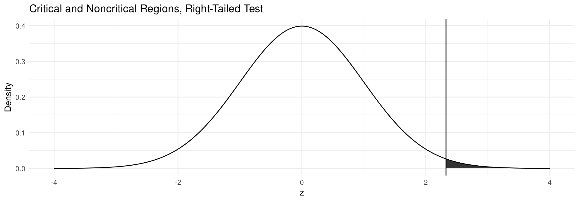
Prepare data — the right-tailed case of Figure 8-5, with \alpha = 0.01.

cv <- qnorm(0.99)
x <- seq(-4, 4, by = 0.01)
curve <- data.frame(x, density = dnorm(x))

cv

[1] 2.326348

Critical and Noncritical Regions in R

Output figure

ggplot(curve, aes(x, density)) +
  geom_area(data = filter(curve, x >= cv)) +
  geom_line() +
  geom_vline(xintercept = cv) +
  labs(title = "Critical and Noncritical Regions, Right-Tailed Test",
       x = "z", y = "Density")

The shaded area to the right of the critical value z = 2.326 is the critical (rejection) region; everything to the left is the noncritical (nonrejection) region.

The Five Steps of Hypothesis Testing

In general a study proceeds by (a) stating the hypotheses, (b) designing the study, (c) conducting the study and collecting the data, (d) evaluating the data, and (e) summarizing the results. Because designing the study and collecting the data are omitted here, a simplified version is used.

Procedure Table: Solving Hypothesis-Testing Problems (Traditional Method)

Step 1. State the hypotheses and identify the claim.

Step 2. Find the critical value(s) from the appropriate table in Appendix A.

Step 3. Compute the test statistic.

Step 4. Make the decision to reject or not reject the null hypothesis.

Step 5. Summarize the results.

Summarizing the Results

Wording the Conclusion

Decision	Claim is H_0	Claim is H_1
Reject H_0	There is enough evidence to reject the claim.	There is enough evidence to support the claim.
Do not reject H_0	There is not enough evidence to reject the claim.	There is not enough evidence to support the claim.

Nothing is proved true or false. The statistician only states that there is, or is not, enough evidence to say that a claim is probably true or false.

The P-Value Method for Hypothesis Testing

P-Value

The P-value (or probability value) is the probability of getting a sample statistic (such as the sample mean) or a more extreme sample statistic in the direction of the alternative hypothesis when the null hypothesis is true.

The P-value is the actual area under the curve of the appropriate distribution representing the probability of the observed sample statistic, or a more extreme one, occurring if H_0 is true.

Comparing \alpha Values and P-Values

Suppose H_1: \mu > 50 and a sample gives \bar{X} = 52. If software reports a P-value of 0.0356, then the probability of getting a sample mean of 52 or greater is 0.0356 when the true population mean is 50. For P = 0.0356, H_0 would be rejected at \alpha = 0.05 but not at \alpha = 0.01.

Caution

When the test is two-tailed, the area in one tail must be doubled. If the area in one tail is 0.0356, the P-value is 2(0.0356) = 0.0712, so H_0 would not be rejected at \alpha = 0.05.

Most calculators and computers report the exact two-tailed P-value already, so it should not be doubled again.

Decision Rule When Using a P-Value

The Rule

If P-value \leq \alpha, reject the null hypothesis.

If P-value > \alpha, do not reject the null hypothesis.

The \alpha value is chosen by the researcher before the statistical test is conducted; the P-value is computed after the sample statistic has been found.

Section 8-2: z Test for a Mean

The General Form of a Test Statistic

General Formula

\text{Test statistic} = \frac{(\text{observed value}) - (\text{expected value})}{\text{standard error}}

The observed value is the statistic computed from the sample data; the expected value is the parameter you would expect if H_0 were true; the denominator is the standard error of the statistic being tested.

The z Test

z Test

The z test is a statistical test for the mean of a population. It can be used either when n \geq 30 or when the population is normally distributed and \sigma is known. The formula for the z test statistic is

z = \frac{\bar{X} - \mu}{\sigma / \sqrt{n}}

where \bar{X} is the sample mean, \mu the hypothesized population mean, \sigma the population standard deviation and n the sample size.

Assumptions and Rounding

Assumptions for the z Test for a Mean When \sigma Is Known

1. The sample is a random sample.
2. Either n \geq 30, or the population is normally distributed when n < 30.

Caution

Test statistics are reported to two or three decimal places so that they are easy to read, but every decision in this chapter is made with the full-precision value R computes. Never round an intermediate result and then keep calculating with the rounded number.

Example 8-3

Basket Size at a Convenience-Store Chain

A category manager believes that the average basket size at her convenience-store chain is now more than the NT$118 reported for last year. Assume the population standard deviation is NT$12. A random sample of 35 transactions has a mean of NT$122.5 (hypothetical data). Test the claim at \alpha = 0.05.

Example 8-3

Solution

Step 1. H_0: \mu = 118 and H_1: \mu > 118 (claim; right-tailed).

Step 2. Since \alpha = 0.05 and the test is right-tailed, the critical value is z = +1.645.

Step 3 — compute the test statistic.

(122.5 - 118) / (12 / sqrt(35))

[1] 2.21853

qnorm(0.95)

[1] 1.644854

Step 4. Since 2.219 is greater than the critical value 1.645, the decision is to reject H_0.

Step 5. There is enough evidence to support the claim that the average basket size is greater than NT$118.

Example 8-4

Island-Wide Parcel Delivery Time

An e-commerce platform states that island-wide parcels arrive on average 48 hours after dispatch. The variable is normally distributed and the population standard deviation is 9 hours. A category manager wishes to see whether parcels in her category arrive significantly faster. She randomly selected 36 parcels and recorded the delivery time in hours, as shown (hypothetical data). At \alpha = 0.10, is there enough evidence to support the claim?

46   52   44   49   41   55
50   43   48   47   39   53
45   51   42   56   38   49
72   44   47   50   46   43
26   48   52   45   49   47
80   41   44   50   30   48

Example 8-4

Solution

Step 1. H_0: \mu = 48 and H_1: \mu < 48 (claim; left-tailed).

Step 2. Since \alpha = 0.10 and the test is left-tailed, the critical value is -1.282.

Step 3 — prepare data and compute the test statistic.

delivery_hours <- c(46, 52, 44, 49, 41, 55,
                    50, 43, 48, 47, 39, 53,
                    45, 51, 42, 56, 38, 49,
                    72, 44, 47, 50, 46, 43,
                    26, 48, 52, 45, 49, 47,
                    80, 41, 44, 50, 30, 48)
x_bar <- mean(delivery_hours)

x_bar

[1] 47.5

(x_bar - 48) / (9 / sqrt(36))

[1] -0.3333333

qnorm(0.10)

[1] -1.281552

Example 8-4

Solution

Step 4. The test statistic -0.333 falls in the noncritical region, so the decision is to not reject H_0.

Step 5. There is not enough evidence to support the claim that parcels in this category arrive faster than the platform average.

Comment. Even though the sample mean 47.5 hours is lower than the hypothesized mean 48 hours, it is not significantly lower; the difference may be due to chance. When H_0 is not rejected, a type II error is still possible, and H_0 cannot be accepted as true — there is merely not enough evidence to say that it is false.

Example 8-5

Checked Baggage on a Regional Route

An airline’s operations report states that checked bags on its Taipei-Tokyo route weigh 18.0 kilograms on average. A load planner selects a random sample of 40 checked bags and finds a mean weight of 19.1 kilograms (hypothetical data). Assume the population standard deviation is 3.0 kilograms. At \alpha = 0.01, can it be concluded that the mean weight is not equal to 18.0 kilograms?

Example 8-5

Solution

Step 1. H_0: \mu = 18 and H_1: \mu \neq 18 (claim; two-tailed).

Step 2. Since \alpha = 0.01 and the test is two-tailed, the critical values are +2.576 and -2.576.

Step 3 — compute the test statistic.

(19.1 - 18) / (3.0 / sqrt(40))

[1] 2.319004

qnorm(0.005)

[1] -2.575829

qnorm(0.995)

[1] 2.575829

Step 4. The test statistic 2.319 falls in the noncritical region, so do not reject H_0.

Step 5. There is not enough evidence to support the claim that the average weight of a checked bag is not equal to 18.0 kilograms.

Procedure Table: The P-Value Method

Solving Hypothesis-Testing Problems (P-Value Method)

Step 1. State the hypotheses and identify the claim.

Step 2. Compute the test statistic.

Step 3. Find the P-value.

Step 4. Make the decision.

Step 5. Summarize the results.

Recall the decision rule: if P-value \leq \alpha, reject H_0; if P-value > \alpha, do not reject H_0.

Example 8-6

Monthly Revenue of a Coffee-Chain Store

A franchise consultant wishes to test the claim that the average monthly revenue of a single coffee-chain store is greater than NT$860 thousand. She selects a random sample of 36 stores and finds the mean to be NT$902 thousand (hypothetical data). The population standard deviation is NT$118 thousand. Is there evidence to support the claim at \alpha = 0.05? Use the P-value method.

Example 8-6

Solution

Step 1. H_0: \mu = 860 and H_1: \mu > 860 (claim; right-tailed).

Step 2 and Step 3 — compute the test statistic and the P-value.

z <- (902 - 860) / (118 / sqrt(36))

z

[1] 2.135593

1 - pnorm(z)

[1] 0.01635629

Step 4. Since the P-value 0.0164 is less than 0.05, reject H_0.

Step 5. There is enough evidence to support the claim that the average monthly revenue of a store is greater than NT$860 thousand. Had \alpha = 0.01 been chosen, H_0 would not have been rejected.

Example 8-7

Courier Pick-Up Time

A food-delivery platform claims that the average time a courier needs to pick up an order from a restaurant is 12 minutes. A sample of 32 pick-ups has an average time of 12.6 minutes (hypothetical data). The standard deviation of the population is 1.9 minutes. At \alpha = 0.05, is there enough evidence to reject the claim? Use the P-value method.

Example 8-7

Solution

Step 1. H_0: \mu = 12 (claim) and H_1: \mu \neq 12 (two-tailed).

Step 2 and Step 3 — compute the test statistic and the P-value.

z <- (12.6 - 12) / (1.9 / sqrt(32))

z

[1] 1.786375

2 * (1 - pnorm(abs(z)))

[1] 0.07403856

Step 4. The decision is to not reject H_0, since the P-value 0.0740 is greater than 0.05.

Step 5. There is not enough evidence to reject the claim that the average pick-up time is 12 minutes.

Guidelines for P-Values

When No \alpha Level Is Chosen

Some researchers report the P-value and let the reader decide. These guidelines can then be used.

• If P-value \leq 0.01, reject the null hypothesis. The difference is highly significant.
• If P-value > 0.01 but P-value \leq 0.05, reject the null hypothesis. The difference is significant.
• If P-value > 0.05 but P-value \leq 0.10, consider the consequences of a type I error before rejecting the null hypothesis.

Section 8-3: t Test for a Mean

The t Distribution

When the population standard deviation is unknown, the z test is not typically used for testing hypotheses involving means; the t test is used instead, and the distribution of the variable should be approximately normal.

How the t Distribution Compares with the Standard Normal

Similarities. It is bell-shaped; it is symmetric about the mean; the mean, median and mode are equal to 0 and are located at the centre of the distribution; the curve approaches but never touches the x axis.

Differences. The variance is greater than 1; it is a family of curves based on the degrees of freedom; as the sample size increases, the t distribution approaches the normal distribution.

The t Test

t Test

The t test is a statistical test for the mean of a population and is used when the population is normally or approximately normally distributed and \sigma is unknown. The formula for the t test statistic is

t = \frac{\bar{X} - \mu}{s / \sqrt{n}}

The degrees of freedom are \text{d.f.} = n - 1.

The formula is the same as for the z test, except that the sample standard deviation s replaces the unknown \sigma.

Reading Table A-5

Caution

Table A-5 gives degrees of freedom for values from 1 through 30, then at intervals above 30. When a critical value is looked up by hand and the degrees of freedom are above 30, round down to the nearest table value — for example, if \text{d.f.} = 59, read \text{d.f.} = 55. This is a conservative approach.

As the degrees of freedom get larger, the critical values approach the z scores. In R, qt() returns the critical value for the exact degrees of freedom, and that is the value quoted on every slide in this chapter; the round-down rule is needed only when the table is read by hand.

Example 8-8

Critical t Value, Right-Tailed

Find the critical t value for \alpha = 0.05 with \text{d.f.} = 19 for a right-tailed t test.

Example 8-8

Solution

Find the 0.05 column in the top row labelled One tail and 19 in the left-hand column. The critical value is +1.729.

qt(0.95, df = 19)

[1] 1.729133

Example 8-9

Critical t Value, Left-Tailed

Find the critical t value for \alpha = 0.01 with \text{d.f.} = 17 for a left-tailed t test.

Example 8-9

Solution

Find the critical value in the 0.01 column in the row labelled One tail, and find 17 in the left column. The critical value is -2.567.

qt(0.01, df = 17)

[1] -2.566934

Example 8-10

Critical t Values, Two-Tailed

Find the critical values for \alpha = 0.05 with \text{d.f.} = 23 for a two-tailed test.

Example 8-10

Solution

Find the 0.05 column in the row labelled Two tails and 23 in the column labelled d.f. The critical values are -2.069 and +2.069.

qt(0.025, df = 23)

[1] -2.068658

qt(0.975, df = 23)

[1] 2.068658

Example 8-11

Critical t Value, Right-Tailed

Find the critical value for \alpha = 0.10 with \text{d.f.} = 12 for a right-tailed test.

Example 8-11

Solution

Find the critical value in the 0.10 column in the One tail row and 12 in the d.f. column. The critical value is +1.356.

qt(0.90, df = 12)

[1] 1.356217

Assumptions for the t Test

Assumptions for the t Test for a Mean When \sigma Is Unknown

1. The sample is a random sample.
2. Either n \geq 30, or the population is normally distributed when n < 30.

Traditional Method with the t Test

The same five steps are used as for the z test, except that critical values come from Table A-5: state the hypotheses and identify the claim; find the critical value(s); compute the test statistic; make the decision; summarize the results.

Example 8-12

Call Handling Time

A customer-service centre claims that the average time an agent needs to handle one call is 4.5 minutes. A random sample of 12 calls had a mean handling time of 5.3 minutes with a standard deviation of 1.1 minutes (hypothetical data). Is there enough evidence to reject the claim at \alpha = 0.05? Assume the variable is normally distributed.

Example 8-12

Solution

Step 1. H_0: \mu = 4.5 (claim) and H_1: \mu \neq 4.5 (two-tailed).

Step 2. The critical values are +2.201 and -2.201 for \alpha = 0.05 and \text{d.f.} = 11.

Step 3 — compute the test statistic.

(5.3 - 4.5) / (1.1 / sqrt(12))

[1] 2.519347

qt(0.975, df = 11)

[1] 2.200985

Step 4. Reject H_0 since 2.519 > 2.201.

Step 5. There is enough evidence to reject the claim that the average call handling time is 4.5 minutes.

Example 8-13

Days to Payment on Export Invoices

An industry report states that small exporters wait on average 27 days to be paid. A trade-finance analyst believes that the exporters using her platform are paid in less time. A random sample of 10 invoices was selected and the number of days to payment is shown (hypothetical data). Test the claim at \alpha = 0.10. Assume the variable is normally distributed.

24   31   19   27   22   30   18   25   21   26

Example 8-13

Solution

Step 1. H_0: \mu = 27 and H_1: \mu < 27 (claim; left-tailed).

Step 2. At \alpha = 0.10 and \text{d.f.} = 9, the critical value is -1.383.

Step 3 — prepare data and compute the test statistic. With the raw data in hand, t.test() does the arithmetic.

days_to_payment <- c(24, 31, 19, 27, 22, 30, 18, 25, 21, 26)

mean(days_to_payment)

[1] 24.3

sd(days_to_payment)

[1] 4.372896

t.test(days_to_payment, mu = 27, alternative = "less")$statistic

        t 
-1.952516 

qt(0.10, df = 9)

[1] -1.383029

Step 4. Reject H_0 since -1.953 falls in the critical region.

Step 5. There is enough evidence to support the claim that exporters on the platform are paid in fewer than 27 days.

P-Value Intervals for the t Test

P-values for t tests cannot be read directly from Table A-5, since only selected values of \alpha are given. Only an interval for the P-value can be found from the table: locate the row for the degrees of freedom, find the two table values the test statistic falls between, and read the corresponding \alpha values from the One tail row (one-tailed test) or the Two tails row (two-tailed test).

Caution

R’s pt() gives the exact P-value. Table A-5 gives only an interval, and the exact value always falls inside that interval. Every decision on these slides is made with the exact value.

Example 8-14

P-Value Interval, Right-Tailed

Find the P-value when the t test statistic is 2.462, the sample size is 14, and the test is right-tailed.

Example 8-14

Solution

Across the row with \text{d.f.} = 13, the value 2.462 falls between 2.160 and 2.650, which correspond to \alpha = 0.025 and \alpha = 0.01 in the One tail row. Hence

0.01 < P\text{-value} < 0.025

1 - pt(2.462, df = 13)

[1] 0.01428067

The exact P-value is 0.0143, which lies inside the interval read from the table. If \alpha were 0.05, H_0 would be rejected; if \alpha were 0.01, it would not.

Example 8-15

P-Value Interval, Two-Tailed

Find the P-value when the t test statistic is 2.575, the sample size is 9, and the test is two-tailed.

Example 8-15

Solution

Across the row with \text{d.f.} = 8, the value 2.575 falls between 2.306 and 2.896, which correspond to \alpha = 0.05 and \alpha = 0.02 in the Two tails row. Hence

0.02 < P\text{-value} < 0.05

2 * (1 - pt(2.575, df = 8))

[1] 0.03287093

The exact P-value is 0.0329. At \alpha = 0.05 the null hypothesis can be rejected; at \alpha = 0.01 it cannot.

Example 8-16

Containers Shipped by Programme Members

A trade association claims that firms which joined its export-promotion programme ship more containers per month than the industry average of 24. A random sample of 15 member firms has a mean of 27.8 containers per month and a standard deviation of 6.2 containers (hypothetical data). Is there enough evidence to support the claim at \alpha = 0.05? Assume the variable is normally distributed. Use the P-value method.

Example 8-16

Solution

Step 1. H_0: \mu = 24 and H_1: \mu > 24 (claim; right-tailed).

Step 2 and Step 3 — compute the test statistic and the P-value.

t_stat <- (27.8 - 24) / (6.2 / sqrt(15))

t_stat

[1] 2.373764

1 - pt(t_stat, df = 14)

[1] 0.01622883

From Table A-5 with \text{d.f.} = 14, the value 2.3738 falls between 2.145 and 2.624, so 0.01 < P\text{-value} < 0.025; the exact P-value is 0.0162.

Step 4. Reject H_0 since P-value < \alpha.

Step 5. There is enough evidence to support the claim that member firms ship more than 24 containers per month.

Choosing Between the z Test and the t Test

Figure 8-23: The Rules

1. If \sigma is known, use the z test. The variable must be normally distributed if n < 30.
2. If \sigma is unknown but n \geq 30, use the t test.
3. If \sigma is unknown and n < 30, use the t test; the population must be approximately normally distributed.

These are the same rules that were used for confidence intervals in Chapter 7.

Section 8-4: z Test for a Proportion

Testing a Proportion

Many hypothesis-testing situations involve proportions; a proportion is the same as a percentage of the population. A hypothesis test involving a population proportion can be considered a binomial experiment when there are only two outcomes and the probability of a success does not change from trial to trial.

Since a normal distribution can be used to approximate the binomial distribution when np \geq 5 and nq \geq 5, the standard normal distribution can be used to test hypotheses for proportions.

Formula for the z Test for Proportions

The Test Statistic

z = \frac{\hat{p} - p}{\sqrt{pq/n}}

where \hat{p} = X/n is the sample proportion, p is the hypothesized population proportion, q = 1 - p and n is the sample size.

The formula follows the general form: \hat{p} is the observed value, p the expected value, and \sqrt{pq/n} the standard error. It is derived from the normal approximation to the binomial by substituting \mu = np and \sigma = \sqrt{npq} and dividing numerator and denominator by n.

Assumptions for Testing a Proportion

Three Assumptions

1. The sample is a random sample.
2. The conditions for a binomial experiment are satisfied.
3. np \geq 5 and nq \geq 5.

Table A-4 is used to find both critical values and P-values. Examples 8-17 to 8-19 use the traditional method; Example 8-20 uses the P-value method.

Example 8-17

Mobile-Wallet Payments

A market-research note claims that 30% of online shoppers in Taiwan pay with a mobile wallet. To test the claim, a student randomly selected 120 online shoppers and found that 42 of them paid with a mobile wallet (hypothetical data). At \alpha = 0.05, is there enough evidence to reject the claim?

Example 8-17

Solution

Step 1. H_0: p = 0.30 (claim) and H_1: p \neq 0.30 (two-tailed).

Step 2. Since \alpha = 0.05 and the test is two-tailed, the critical values are \pm 1.960.

Step 3 — compute the test statistic.

p_hat <- 42 / 120

p_hat

[1] 0.35

(p_hat - 0.30) / sqrt(0.30 * 0.70 / 120)

[1] 1.195229

qnorm(0.975)

[1] 1.959964

Step 4. Do not reject H_0, since the test statistic 1.195 falls in the noncritical region.

Step 5. There is not enough evidence to reject the claim that 30% of online shoppers pay with a mobile wallet.

Example 8-18

Night-Market Stalls Accepting Mobile Payment

An industry survey reports that 40% of night-market stalls accept mobile payment. A researcher believes that the percentage is lower at one particular night market. She randomly selected 60 stalls there and found that 20 accept mobile payment (hypothetical data). At \alpha = 0.01, is there enough evidence to support the claim?

Example 8-18

Solution

Step 1. H_0: p = 0.40 and H_1: p < 0.40 (claim; left-tailed).

Step 2. Since \alpha = 0.01 and the test is one-tailed, the critical value is -2.326.

Step 3 — compute the test statistic.

p_hat <- 20 / 60

p_hat

[1] 0.3333333

(p_hat - 0.40) / sqrt(0.40 * 0.60 / 60)

[1] -1.054093

qnorm(0.01)

[1] -2.326348

Step 4. Do not reject H_0, since the test statistic -1.054 does not fall in the critical region.

Step 5. There is not enough evidence to support the claim that fewer than 40% of the stalls at this night market accept mobile payment.

Example 8-19

Booking Accommodation Online

A tourism report states that at least 72% of inbound visitors to Taiwan book their accommodation online. To see whether this claim is valid, a researcher selected a random sample of 90 inbound visitors and found that 60 of them had booked online (hypothetical data). At \alpha = 0.01, test the claim that at least 72% of inbound visitors book their accommodation online.

Example 8-19

Solution

Step 1. H_0: p = 0.72 (claim) and H_1: p < 0.72 (left-tailed).

Step 2. Since \alpha = 0.01 and the test is left-tailed, the critical value is -2.326.

Step 3 — compute the test statistic.

p_hat <- 60 / 90

p_hat

[1] 0.6666667

(p_hat - 0.72) / sqrt(0.72 * 0.28 / 90)

[1] -1.126872

qnorm(0.01)

[1] -2.326348

Step 4. Do not reject H_0, since the test statistic -1.127 does not fall in the critical region.

Step 5. There is not enough evidence to reject the claim that at least 72% of inbound visitors book their accommodation online.

Example 8-20

Cross-Border Orders Shipped to Japan

A payments company claims that more than 20% of the cross-border e-commerce orders placed from Taiwan are shipped to Japan. A random sample of 250 cross-border orders showed that 63 were shipped to Japan (hypothetical data). At \alpha = 0.05, is there enough evidence to support the claim? Use the P-value method.

Example 8-20

Solution

Step 1. H_0: p = 0.20 and H_1: p > 0.20 (claim; right-tailed).

Step 2 and Step 3 — compute the test statistic and the P-value.

p_hat <- 63 / 250
z     <- (p_hat - 0.20) / sqrt(0.20 * 0.80 / 250)

p_hat

[1] 0.252

z

[1] 2.05548

1 - pnorm(z)

[1] 0.01991631

Step 4. Reject H_0, since the P-value 0.0199 is less than 0.05.

Step 5. There is enough evidence to support the claim that more than 20% of the cross-border orders placed from Taiwan are shipped to Japan.

Finding Chi-Square Critical Values

Three Cases Using Table A-6

Table A-6 gives the areas to the right of the critical value.

1. Right-tailed test — use the area under the \alpha value for the specific degrees of freedom.
2. Left-tailed test — subtract \alpha from 1, then use the area for 1 - \alpha.
3. Two-tailed test — divide \alpha by 2; use the area for \alpha/2 for the right critical value and the area for 1 - \alpha/2 for the left critical value.

In R, qchisq(area, df) returns the value with area to its left, which is why the arguments below are 1 - \alpha, \alpha, and so on.

Example 8-21

Critical Chi-Square Value, Right-Tailed

Find the critical chi-square value for 18 degrees of freedom when \alpha = 0.05 and the test is right-tailed.

Example 8-21

Solution

Find the \alpha value at the top of Table A-6 and the degrees of freedom in the left column. The critical value is located where the two columns meet: 28.869.

qchisq(0.95, df = 18)

[1] 28.8693

Example 8-22

Critical Chi-Square Value, Left-Tailed

Find the critical chi-square value for 14 degrees of freedom when \alpha = 0.05 and the test is left-tailed.

Example 8-22

Solution

When the test is left-tailed, the \alpha value must be subtracted from 1: 1 - 0.05 = 0.95. The chi-square table gives the area to the right of the critical value, and chi-square values cannot be negative, so 95% of the area will be to the right of the value. For 0.95 and 14 degrees of freedom the critical value is 6.571.

qchisq(0.05, df = 14)

[1] 6.570631

Example 8-23

Critical Chi-Square Values, Two-Tailed

Find the critical chi-square values for 19 degrees of freedom when \alpha = 0.10 and a two-tailed test is conducted.

Example 8-23

Solution

The area must be split: the area to the right of the larger value is \alpha/2 = 0.05, and the area to the right of the smaller value is 1 - \alpha/2 = 0.95. With 19 degrees of freedom the critical values are 10.117 and 30.144.

qchisq(0.05, df = 19)

[1] 10.11701

qchisq(0.95, df = 19)

[1] 30.14353

Degrees of Freedom Beyond the Table

Caution

Table A-6 gives values only up to 30 degrees of freedom. When the degrees of freedom exceed those specified in the table, use the table value for 30 degrees of freedom. This guideline keeps the type I error equal to or below the \alpha value.

Three Test Situations for a Variance

If a researcher believes the variance of a population is greater than 225: H_0: \sigma^2 = 225 and H_1: \sigma^2 > 225 — right-tailed.

If less than 225: H_0: \sigma^2 = 225 and H_1: \sigma^2 < 225 — left-tailed.

If no direction is specified: H_0: \sigma^2 = 225 and H_1: \sigma^2 \neq 225 — two-tailed.

The Chi-Square Test for a Single Variance

Formula

\chi^2 = \frac{(n-1)s^2}{\sigma^2}

with degrees of freedom equal to n - 1, where n is the sample size, s^2 the sample variance and \sigma^2 the population variance.

Assumptions for the Chi-Square Test for a Single Variance

1. The sample must be randomly selected from the population.
2. The population must be normally distributed for the variable under study.
3. The observations must be independent of one another.

Why Test a Variance?

Wherever consistency is required, the smallest possible variation is wanted. When bolts are manufactured, the variation in diameters must be kept to a minimum, or the nuts will not fit properly. In education, a test used repeatedly on the same students should produce approximately the same grades, so the variance of each student’s grades should be small — but a test used to judge learning should have a large overall standard deviation, so that those who have learned can be distinguished from those who have not.

Caution

The methods used to test a hypothesis about a population variance or standard deviation are not robust. If the data come from a population that is not normally distributed, these methods cannot be used.

Example 8-24

Fill Weight of Snack Packs

A quality engineer wishes to see whether the variance of the fill weight of a snack pack on one production line is less than the process standard of \sigma^2 = 36 (grams squared). A random sample of 12 packs from that line had a variance of s^2 = 27 (hypothetical data). Test her claim at \alpha = 0.05.

Example 8-24

Solution

Step 1. H_0: \sigma^2 = 36 and H_1: \sigma^2 < 36 (claim; left-tailed).

Step 2. Since this is a left-tailed test and \alpha = 0.05, the value 1 - 0.05 = 0.95 is used with \text{d.f.} = 11. The critical value is 4.575.

Step 3 — compute the test statistic.

(12 - 1) * 27 / 36

[1] 8.25

qchisq(0.05, df = 11)

[1] 4.574813

Step 4. Since 8.250 falls in the noncritical region, do not reject H_0.

Step 5. There is not enough evidence to support the claim that the variance of the fill weight on this line is less than 36.

Example 8-25

Orders Picked per Hour

A distribution-centre manager believes that the standard deviation of the number of orders picked per hour is greater than 6. A random sample of 15 hours is selected and the number of orders picked in each hour is shown (hypothetical data). At \alpha = 0.10, is there enough evidence to support the manager’s claim? Assume the variable is normally distributed.

38   52   45   61   40
55   33   48   57   42
36   50   65   44   39

Example 8-25

Solution

Step 1. H_0: \sigma = 6 and H_1: \sigma > 6 (claim; right-tailed). Since the standard deviation is given, it is squared to get the variance.

Step 2. Right-tailed with \text{d.f.} = 14 and \alpha = 0.10: the critical value is 21.064.

Step 3 — prepare data and compute the test statistic.

orders_per_hour <- c(38, 52, 45, 61, 40,
                     55, 33, 48, 57, 42,
                     36, 50, 65, 44, 39)

sd(orders_per_hour)

[1] 9.516902

(15 - 1) * var(orders_per_hour) / 6^2

[1] 35.22222

qchisq(0.90, df = 14)

[1] 21.06414

Step 4. Reject H_0, since 35.222 > 21.064.

Step 5. There is enough evidence to support the claim that the standard deviation of the number of orders picked per hour is greater than 6.

Example 8-26

Net Weight of Instant-Noodle Packs

A contract manufacturer wishes to test the claim that the variance of the net weight of its instant-noodle packs is 2.25. Net weight is measured in grams, and assume that it is normally distributed. A random sample of 20 packs has a standard deviation of 1.8 grams (hypothetical data). At \alpha = 0.05, is there enough evidence to reject the manufacturer’s claim?

Example 8-26

Solution

Step 1. H_0: \sigma^2 = 2.25 (claim) and H_1: \sigma^2 \neq 2.25 (two-tailed).

Step 2. Two-tailed at \alpha = 0.05, so the critical values for 0.025 and 0.975 are needed. With \text{d.f.} = 19 they are 8.907 and 32.852.

Step 3 — compute the test statistic. Since the sample standard deviation is given, it must be squared for the formula.

(20 - 1) * 1.8^2 / 2.25

[1] 27.36

qchisq(0.025, df = 19)

[1] 8.906516

qchisq(0.975, df = 19)

[1] 32.85233

Step 4. Do not reject H_0, since 8.907 < 27.360 < 32.852.

Step 5. There is not enough evidence to reject the manufacturer’s claim that the variance of the net weight is equal to 2.25.

P-Value Intervals for the Chi-Square Test

Approximate P-values for the chi-square test can be found from Table A-6, but the procedure is more complicated than for the z and t tests, since the chi-square distribution is not symmetric and \chi^2 values cannot be negative.

Reading the Interval

• Right-tailed. Find the two table values the test statistic falls between and read the corresponding \alpha values directly.
• Left-tailed. Read the corresponding table values, then subtract each from 1.
• Two-tailed. Find the interval as above, then double both endpoints.

Example 8-27

P-Value Interval, Right-Tailed

Find the P-value when \chi^2 = 21.5, n = 11, and the test is right-tailed.

Example 8-27

Solution

Across the row with \text{d.f.} = 10, the value 21.5 falls between 20.483 and 23.209, corresponding to 0.025 and 0.01 respectively. Hence

0.01 < P\text{-value} < 0.025

1 - pchisq(21.5, df = 10)

[1] 0.01786459

The exact P-value is 0.0179, which lies inside that interval.

Example 8-28

P-Value Interval, Left-Tailed

Find the P-value when \chi^2 = 5.892, n = 15, and the test is left-tailed.

Example 8-28

Solution

Across the row with \text{d.f.} = 14, the value 5.892 falls between 5.629 and 6.571, corresponding to 0.975 and 0.95. Because the test statistic falls on the left side, each value must be subtracted from 1: 1 - 0.975 = 0.025 and 1 - 0.95 = 0.05. Hence

0.025 < P\text{-value} < 0.05

pchisq(5.892, df = 14)

[1] 0.03085947

The exact P-value is 0.0309. Had the test been two-tailed, the interval would be doubled: 0.05 < P\text{-value} < 0.10.

Example 8-29

Customs Clearance Times

A customs broker knows from past records that the standard deviation of the time needed to clear an import container is 9.5 hours. A random sample of 25 containers is selected and timed; the standard deviation is 7.0 hours (hypothetical data). At \alpha = 0.05, can it be concluded that the standard deviation has changed? Use the P-value method. Assume the variable is normally distributed.

Example 8-29

Solution

Step 1. H_0: \sigma = 9.5 and H_1: \sigma \neq 9.5 (claim; two-tailed).

Step 2 and Step 3 — compute the test statistic and the P-value.

chi_sq <- (25 - 1) * 7.0^2 / 9.5^2

chi_sq

[1] 13.03047

2 * pchisq(chi_sq, df = 24)

[1] 0.06876872

With \text{d.f.} = 24, the value 13.0305 falls between 12.401 and 13.848, corresponding to 0.975 and 0.95. Subtracting from 1 gives 0.025 and 0.05, and doubling for the two tails gives 0.05 < P\text{-value} < 0.10; the exact P-value is 0.0688.

Step 4. Do not reject H_0, since P-value > \alpha.

Step 5. There is not enough evidence to support the claim that the standard deviation of the customs clearance time has changed.

Example 8-30

Value of Air-Freight Shipments

A trade magazine reports that the average declared value of an air-freight shipment leaving Taoyuan is NT$68 thousand. A freight forwarder randomly selected 50 recent shipments and found that the average declared value was NT$63.8 thousand and the standard deviation was NT$9.6 thousand (hypothetical data). Is there enough evidence at \alpha = 0.05 to conclude that the average value is not NT$68 thousand? Assume the variable is normally distributed. Also find the 95% confidence interval of the true mean.

Example 8-30

Solution

Step 1. H_0: \mu = 68 and H_1: \mu \neq 68 (claim; two-tailed).

Step 2. At \alpha = 0.05 with \text{d.f.} = 49, qt() gives the critical values +2.010 and -2.010.

Step 3 — compute the test statistic.

(63.8 - 68) / (9.6 / sqrt(50))

[1] -3.093592

qt(0.975, df = 49)

[1] 2.009575

Step 4. Since -3.094 < -2.010, the decision is to reject H_0.

Step 5. There is enough evidence to support the claim that the average declared value is not NT$68 thousand.

Example 8-30

Solution

The 95% confidence interval.

\bar{X} - t_{\alpha/2}\frac{s}{\sqrt{n}} < \mu < \bar{X} + t_{\alpha/2}\frac{s}{\sqrt{n}}

margin <- qt(0.975, df = 49) * 9.6 / sqrt(50)

63.8 - margin

[1] 61.07171

63.8 + margin

[1] 66.52829

The interval 61.07 < \mu < 66.53 does not contain the hypothesized value \mu = 68. There is agreement between the hypothesis test and the confidence interval.

Example 8-31

Net Weight of Tea-Bag Cartons

A supplier claims that its cartons of tea bags have an average net weight of 120 grams. A random sample of 10 cartons has an average net weight of 118.6 grams and a standard deviation of 2.8 grams (hypothetical data). At \alpha = 0.05, can the claim be rejected? Also, find the 95% confidence interval of the true mean. Assume the variable is normally distributed.

Example 8-31

Solution

Step 1. H_0: \mu = 120 (claim) and H_1: \mu \neq 120 (two-tailed).

Step 2. At \alpha = 0.05 and \text{d.f.} = 9, the critical values are +2.262 and -2.262.

Step 3 — compute the test statistic and the interval.

margin <- qt(0.975, df = 9) * 2.8 / sqrt(10)

(118.6 - 120) / (2.8 / sqrt(10))

[1] -1.581139

qt(0.975, df = 9)

[1] 2.262157

118.6 - margin

[1] 116.597

118.6 + margin

[1] 120.603

Step 4 and Step 5. Do not reject H_0. There is not enough evidence to reject the claim that the mean net weight is 120 grams. The 95% interval 116.6 < \mu < 120.6 does contain \mu = 120; again there is agreement.

Type II Error and the Power of a Test

Figure 8-40: Possibilities in Hypothesis Testing

Decision	H_0 true	H_0 false
Reject H_0	Type I error, \alpha	Correct decision, 1 - \beta
Do not reject H_0	Correct decision, 1 - \alpha	Type II error, \beta

The value of \beta depends on \alpha, the sample size, the population standard deviation, and the actual difference between the hypothesized parameter and the true parameter. Since that last difference is unknown, \beta cannot be computed.

The Power of a Test

Power of a Test

The power of a statistical test measures the sensitivity of the test to detect a real difference in parameters if one actually exists. The power of a test is equal to

\text{Power} = 1 - \beta

Power is a probability and can take values from 0 to 1. The closer the power is to 1, the better the test is at rejecting the null hypothesis when the null hypothesis is in fact false. If \beta = 0.04, the power is 1 - 0.04 = 0.96, or 96%.

Increasing the Power of a Test

Two Practical Methods

1. Increase \alpha — for example use \alpha = 0.05 instead of \alpha = 0.01. As \alpha increases, \beta decreases, so 1 - \beta increases.
2. Select a larger sample size — a larger n makes the standard error of the mean smaller and consequently reduces \beta.

Neither should be used at the researcher’s whim. Before increasing \alpha, consider the consequences of a type I error; increasing the sample size costs money and time.

When a choice of statistical tests exists, use the test with the highest power for the data — provided its assumptions can be met. If they cannot, a test with lower power must be used.

Power in R

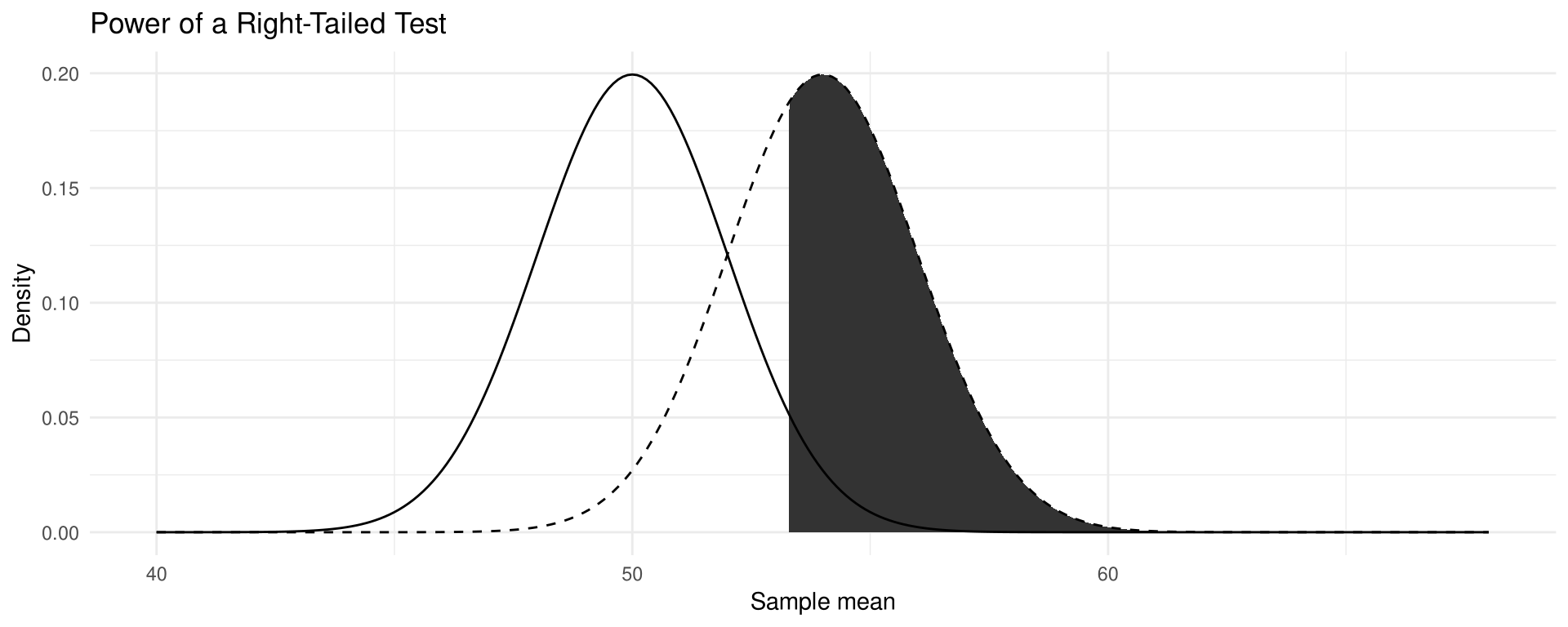
Prepare data — the distribution of \bar{X} under H_0: \mu = 50 and under the true value \mu = 54, with \sigma = 10, n = 25 and a right-tailed test at \alpha = 0.05.

se   <- 10 / sqrt(25)
cv   <- 50 + qnorm(0.95) * se
beta <- pnorm(cv, 54, se)

cv

[1] 53.28971

beta

[1] 0.36124

1 - beta

[1] 0.63876

x <- seq(40, 68, by = 0.1)
curves <- data.frame(x, h0 = dnorm(x, 50, se), h1 = dnorm(x, 54, se))

Power in R

Output figure

ggplot(curves, aes(x)) +
  geom_area(data = filter(curves, x >= cv), aes(y = h1)) +
  geom_line(aes(y = h0)) +
  geom_line(aes(y = h1), linetype = "dashed") +
  labs(title = "Power of a Right-Tailed Test", x = "Sample mean", y = "Density")

The solid curve is for H_0: \mu = 50 and the dashed curve for the true value \mu = 54. The shaded area is the power 1 - \beta = 0.639; the unshaded part of the dashed curve is \beta = 0.361. Increasing n narrows both curves and increases the power.

A Final Comment

Caution

When the researcher fails to reject the null hypothesis, this does not mean that there is not enough evidence to support alternative hypotheses. It may be that the null hypothesis is false but the statistical test has too low a power to detect the real difference. One can conclude only that in this study there is not enough evidence to reject the null hypothesis.

Whether the decision is to reject H_0 or not to reject H_0, there is in either case a chance of being wrong. The goal is to keep the probabilities of type I and type II errors as small as possible.

Important Terms

Chapter 8 Vocabulary

\alpha (alpha) · alternative hypothesis · \beta (beta) · chi-square test · critical or rejection region · critical value · hypothesis testing · left-tailed test · level of significance · noncritical or nonrejection region · null hypothesis · one-tailed test · power of a test · P-value · research hypothesis · right-tailed test · statistical hypothesis · statistical test · test statistic · t test · two-tailed test · type I error · type II error · z test

Key Formulas

Tests for Means

The general form of a test statistic:

\text{Test statistic} = \frac{(\text{observed value}) - (\text{expected value})}{\text{standard error}}

The z test for means — if n < 30, the variable must be normally distributed:

z = \frac{\bar{X} - \mu}{\sigma / \sqrt{n}}

The t test for means, \text{d.f.} = n - 1 — if n < 30, the variable must be normally distributed:

t = \frac{\bar{X} - \mu}{s / \sqrt{n}}

Key Formulas

Tests for Proportions, Variances and Standard Deviations

The z test for proportions, valid if np \geq 5 and nq \geq 5, where \hat{p} = X/n and q = 1 - p:

z = \frac{\hat{p} - p}{\sqrt{pq/n}}

The chi-square test for a variance or standard deviation, \text{d.f.} = n - 1 — the variable must be normally distributed:

\chi^2 = \frac{(n-1)s^2}{\sigma^2}

The power of a test:

\text{Power} = 1 - \beta

Key Takeaways

Key point

• A statistical hypothesis is a conjecture about a population parameter; H_0 states no difference and always carries the equals sign, while H_1 states a difference and is also called the research hypothesis
• Evidence can support a claim only when the claim is H_1, and can reject a claim only when the claim is H_0; nothing is ever proved
• A type I error rejects a true H_0 and has probability \alpha, the level of significance; a type II error fails to reject a false H_0 and has probability \beta — decreasing one increases the other
• The critical value separates the critical (rejection) region from the noncritical (nonrejection) region; the direction of H_1 decides whether the test is left-tailed, right-tailed or two-tailed
• Traditional method: state the hypotheses and identify the claim, find the critical value(s), compute the test statistic, make the decision, summarize the results

Key Takeaways

Key point

• P-value method: state the hypotheses and identify the claim, compute the test statistic, find the P-value, make the decision, summarize the results — reject H_0 when P-value \leq \alpha
• Use the z test when \sigma is known, the t test with \text{d.f.} = n - 1 when \sigma is unknown; test a proportion with z when np \geq 5 and nq \geq 5, and a variance with \chi^2 when the population is normal
• For a two-tailed test, the (1 - \alpha) confidence interval contains the hypothesized value exactly when H_0 is not rejected
• The power of a test is 1 - \beta; it is raised by increasing \alpha or, better, by increasing the sample size

Acknowledgement

• Copyright notice. These teaching materials follow the organization and terminology of Bluman, A. G. (2023). Elementary statistics: A step by step approach (11th ed.). McGraw Hill. All rights in the original work are reserved by its authors and publishers.

• Original examples. Every worked example, data set, and R script in these slides was written for this course. The data are hypothetical unless stated otherwise.

• Non-commercial use only. These materials are strictly intended for educational purposes and must not be used for commercial gain or profit.

• Proper attribution. Any reproduction, distribution, or use of these materials must provide proper attribution to the original source.